Forward-Backward prediction

What happens if we do fully causal prediction, but in the backward direction—so last-word-first—in addition to causal prediction forward?

Answer: Only a $5\%$ chance of doing a backward prediction in addition to a forward prediction during training is enough for the model to learn the backward task almost perfectly. And in large enough models, it also doesn’t degrade performance on the forward task (the trend is actually towards it improving forward performace at sufficient scale).

Code under snimu/mask.

Terminology

• fw task/prediction: Short for the forward task/prediction
• bw task/prediction: Short for the backward task/prediction
• $p_{bw}$: The probability of doing a bw prediction in addition to a fw prediction (see Methods)

Why?

I can see three potential advantages of training on the bw task:

1. Forcing the model to learn to distinguish between a fw and bw causal mask, and adjust properly, may serve as a form of dataset augmentation that effectively increases the data diversity, and thus allows a model to learn more from the same data than otherwise possible.
2. You have a model that can perform the bw task. That might be useful.
3. Masked prediction for RAG / infilling. This is pure speculation and I didn’t test it, but models trained with a bit of the bw task might be easier to finetune into RAG models with a bidirectional mask than fw-task-only ones. This is especially true if combined with MEAP, which does causal prediction on masked input sequences. This, combined with backward prediction, would make the model much closer to a bidirectional Masked Language Model (MLM).

Methods

I trained hlb-gpt v0.4.1 for 10 epochs on wikitext. I perform the fw task and, with probability $p_{bw}$, also the bw task on the same tokens. I accumulate the losses and then do a backward pass. Why didn’t I do either only a fw or only a bw prediction at the same time? Well, I should have; but this is an old project that I’m just now re-visiting, and that’s the choice I made back then.

Inspired by Yi Tay et al.’s UL2, I’ve informed the models of their task by giving them a special token at the beginning of text if I’m fw masking or a different one at the end of the text if I’m bw masking.

I do this for different model sizes: I trained three models for every combination of depth in ${4, 8, 16, 32}$ and width in ${192, 384, 768, 1536}$. This is done for different values of $p_{bw}$: $0\%$ and $5\%$ (in early testing, higher probabilities degraded fw performance too much; more on that later).

After a model is trained for 10 epochs, I remove the transformer layers one by one, starting from the back, and evaluate the resulting model after each removal. I hope that this gives me some insights into which parts of the model are more important for the fw and bw predictions, respectively. My first hypothesis was that early layers are used to distinguish between the fw and bw task, and thus the positive effects of dual masking can only occur in deep networks that can make use of the knowledge extracted in the early layers.

Per setting (depth, width, $p_bw$, or using fw mask only), I train three times. I’ve saved all results, but below, will only show you the average over all three runs for each setting.

Background info

Unless specifically stated otherwise, $p_{bw} = 5\%$ for all experiments where $p_{bw}$ is non-zero, because with $p_{bw} = 10\%$, the relative performance between models trained with the fw-mask only and those trained with a bidirectional mask was very skewed towards the fw-only models.

Metrics

Besides the obvious metrics, like validation loss or accuracy, I look at two ratios that are very telling:

1. ratio 1: $\frac{\mathrm{metric-fw}{p{bw} = 0\%}}{\mathrm{metric-fw}{p{bw} = 5\%}}$

   The models trained with $p_{bw} > 0\%$ are obviously better at the bw prediction than the ones trained with $p_{bw} = 0\%$. What I’m interested in here is how a non-zero $p_{bw}$ impacts the fw performance of the models. This ratio is the performance for $p_{bw} = 0\%$ divided by the performance for $p_{bw} = x\%$, where $x$ is usually $5$, and the metric-fw is usually just the fw validation loss.

2. ratio 2: $\frac{\mathrm{metric-fw}{p{bw} \ge 0 \%}}{\mathrm{metric-bw}{p{bw} \ge 0\%}}$

   How much better is a model at the fw task than the bw task? Lower obviously means better fw, while higher means better bw performance. This will be interesting when looking at performance with layers removed.

For both, I have two ways to calculate the average ratio over several runs:

1. First calculate the means of the metric over the three runs I want to average, then calculate the ratio. This will squash outliers. I will call it mean_then_ratio.
2. First calculate the individual ratios per step, then average them over the three runs. This measure is more receptive to outliers. I will call it ratio_then_mean.

Performance for different widths

To get a feel for how training evolves for different $p_{bw}$ at different model scales, let’s first look at the fw and bw validation loss for the default model size in hlb-gpt:

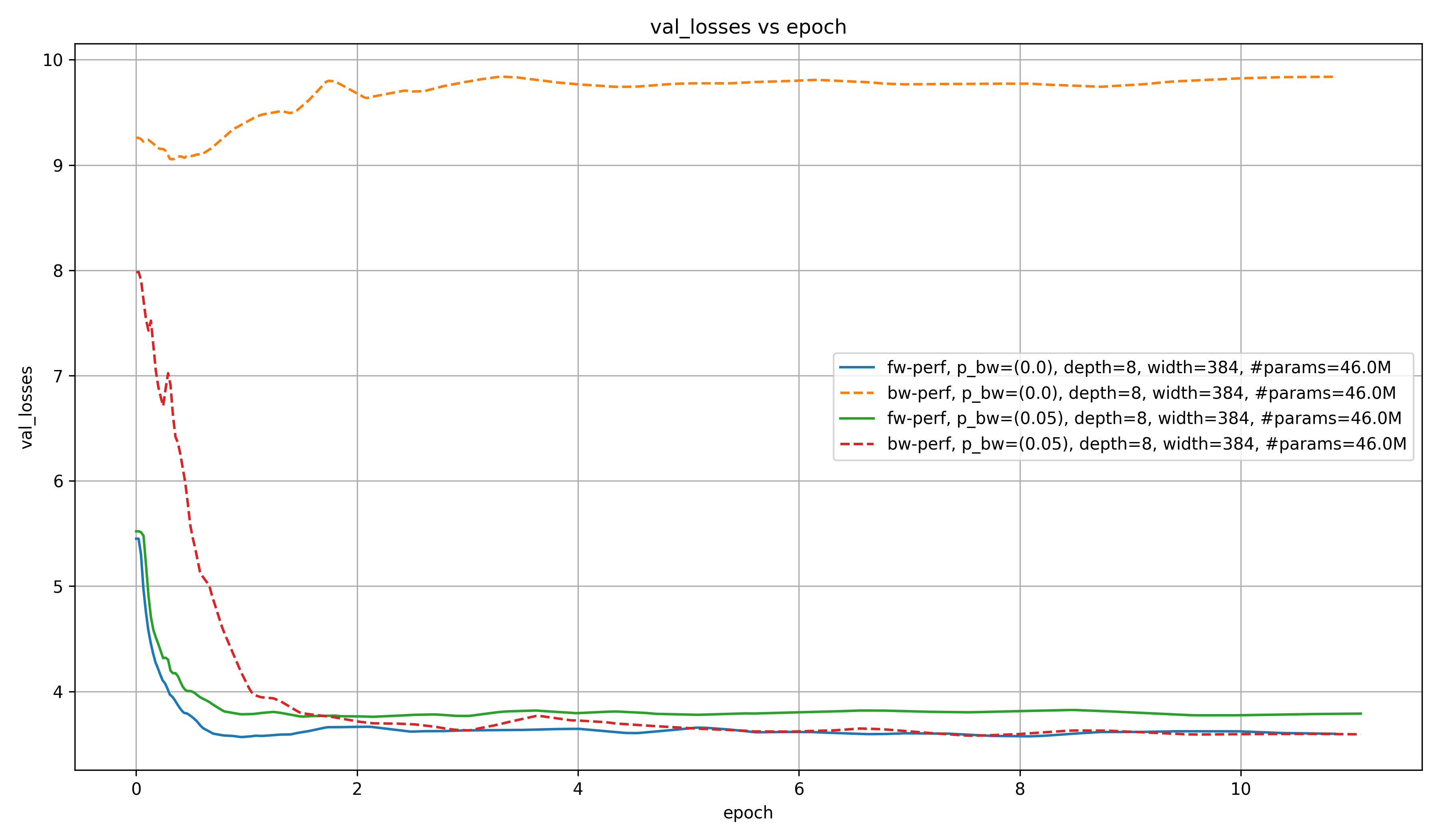
As you can see, the fw loss is lower in the model trained only on the fw task than for the one trained on both the fw and the bw task, even after $10$ epochs. As we will see later, this likely changes with scale.

It is also very obvious, however, that even a small $p_{bw}$ of $5\%$ will lead to a very loss bw loss, while the bw loss actually increases for the models trained with $p_{bw} = 0\%$. This is a nice validation that something is working as intended, and the intended benefits for downstream RAG tasks may actually come true.

Now, let’s look at how this behaves for different model scales.

Performance by model scale

Below, I show the ratio 1 between the fw performance of models trained with $p_{bw} = 0\%$ compared to those trained with $p_{bw} = 5\%$ (as described above under Metrics) for models of different width and depth, as well as over the combined number of parameters.

I compute the ratio independently for each of the training runs per setting, and independently for each of $500$ steps over the approximately $10$ epochs. In other words, I don’t just take the ratio at the last step, but over every step in the entire training-run; each as its own sample. (for details, see the code provided in plot_results.py).

Then, take the ratios falling into the range $\left[\mathrm{epoch}{\mathrm{start}}, \mathrm{epoch}{\mathrm{stop}}\right]$ and plot them as a boxplot or violinplot.

Below, you can see the violinplot for all available data ($\mathrm{epoch}{\mathrm{start}} = 0, \mathrm{epoch}{\mathrm{stop}} = 10$):

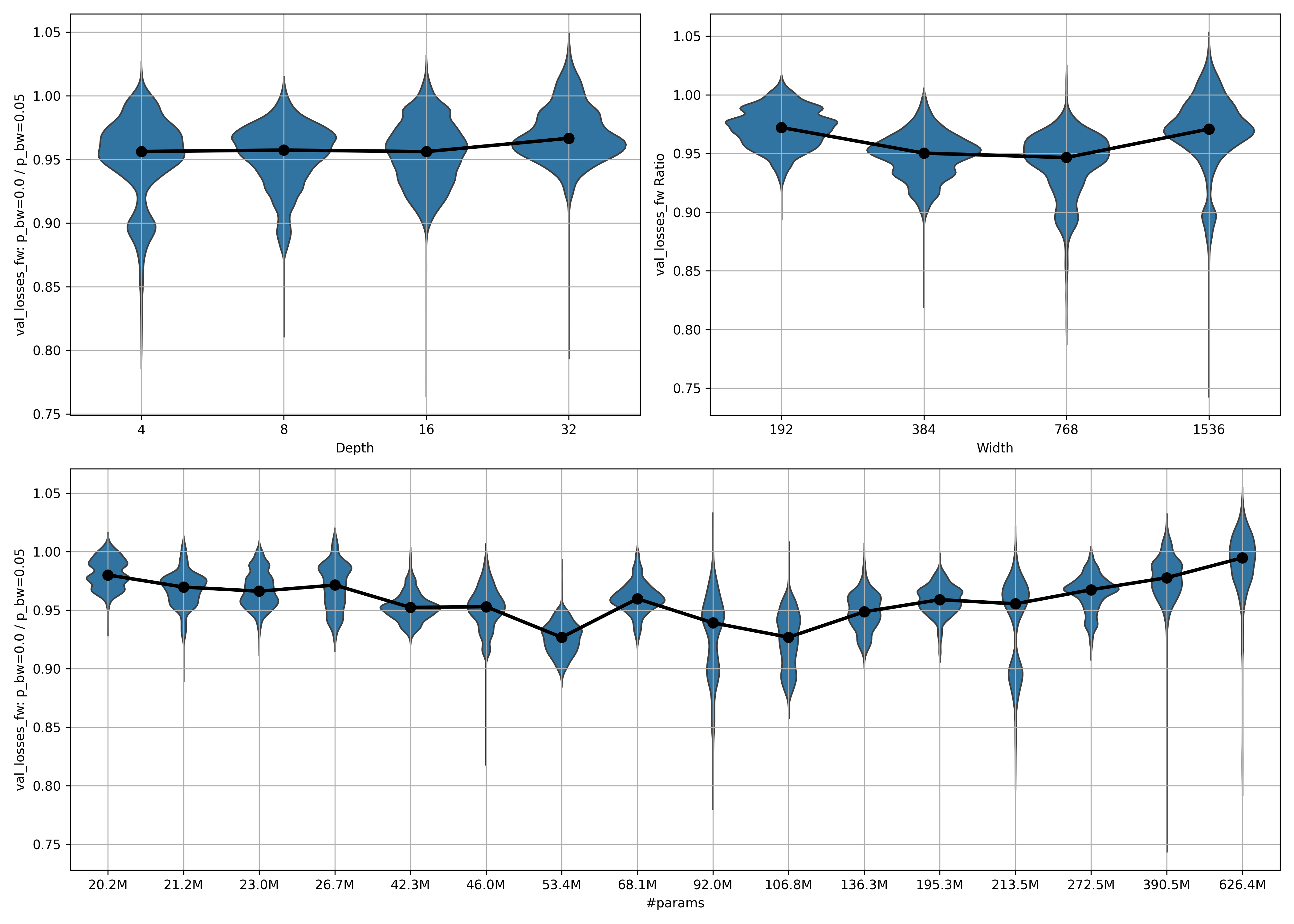
A few thoughts:

• There seems to be an inverse scaling law for small model sizes, reminiscent of Better & Faster Large Language Models via Multi-token Prediction. This has its minimum at $106.8$ million parameters.
• Beyond that, positive scaling laws apply. As the number of parameters grows, the ratio increases as well, meaning that the models trained with $p_{bw} = 5\%$ are catching up in fw performance to the models trained with $p_{bw} = 0\%$.
• In the largest model, performance has caught up. This is fantastic! It implies that with the model sizes common today, using $p_{bw} = 5\%$ at worst doesn’t negatively impact fw performance, while unlocking bw capabilities, and at best positively impacts fw performance.
• This scaling law—first inverse, then normal—applies more strongly to the width than to the depth.

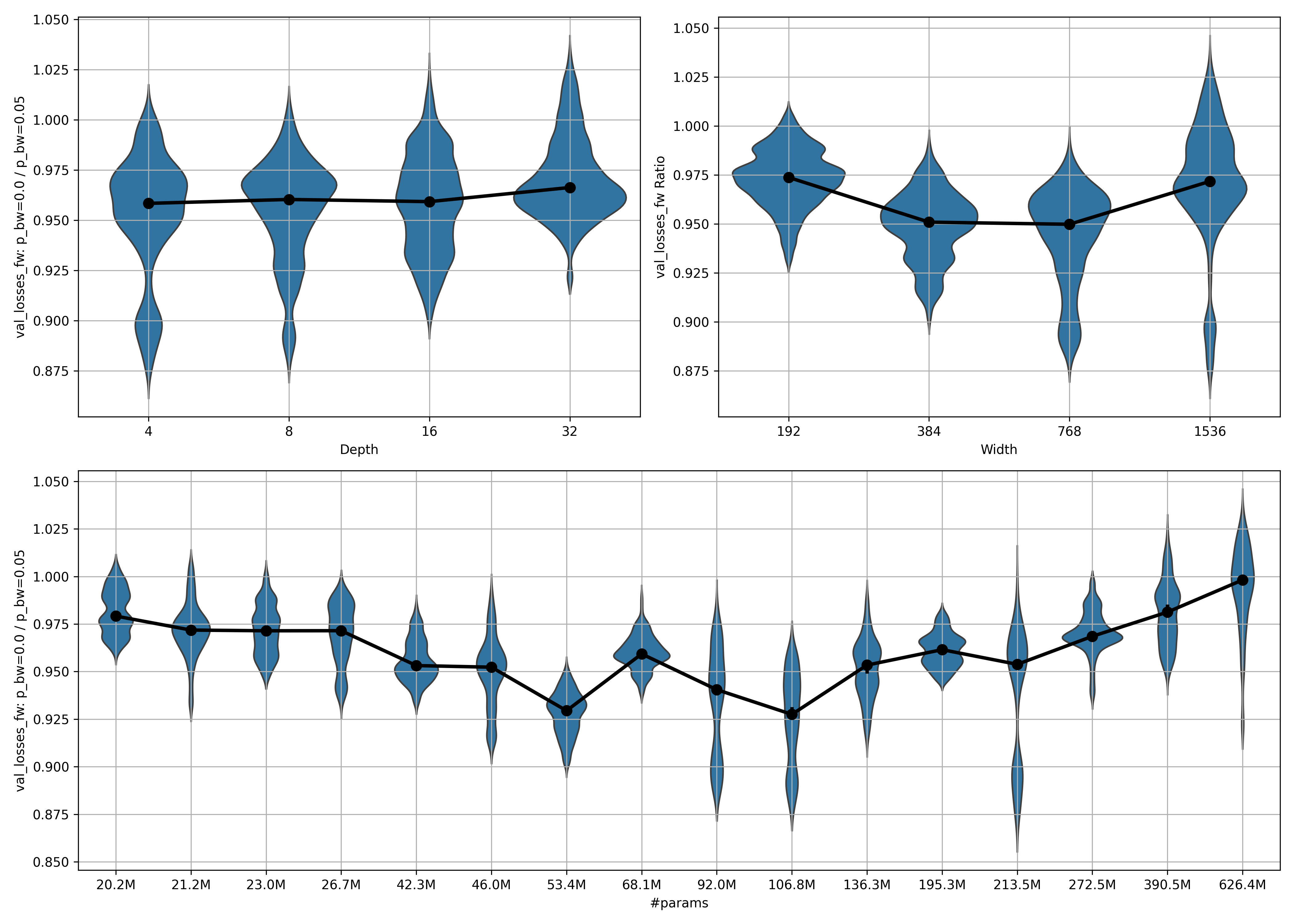
So how does this apply at different epochs during training? Here is the violinplot of ratio 1 for only the first epoch ($\mathrm{epoch}{\mathrm{start}} = 0, \mathrm{epoch}{\mathrm{stop}} = 1$):

It looks like in the first epoch, even the largest model has a ratio significantly below $1$. This implies that it takes many samples for the models trained with $p_{bw} = 5\%$ to catch up to those trained with $p_{bw} = 0\%$ in fw performance. Alternatively, it might mean that this is a regularization technique that is useful only for training for many epochs. It might be interesting to try this on a more serious dataset than wikitext.

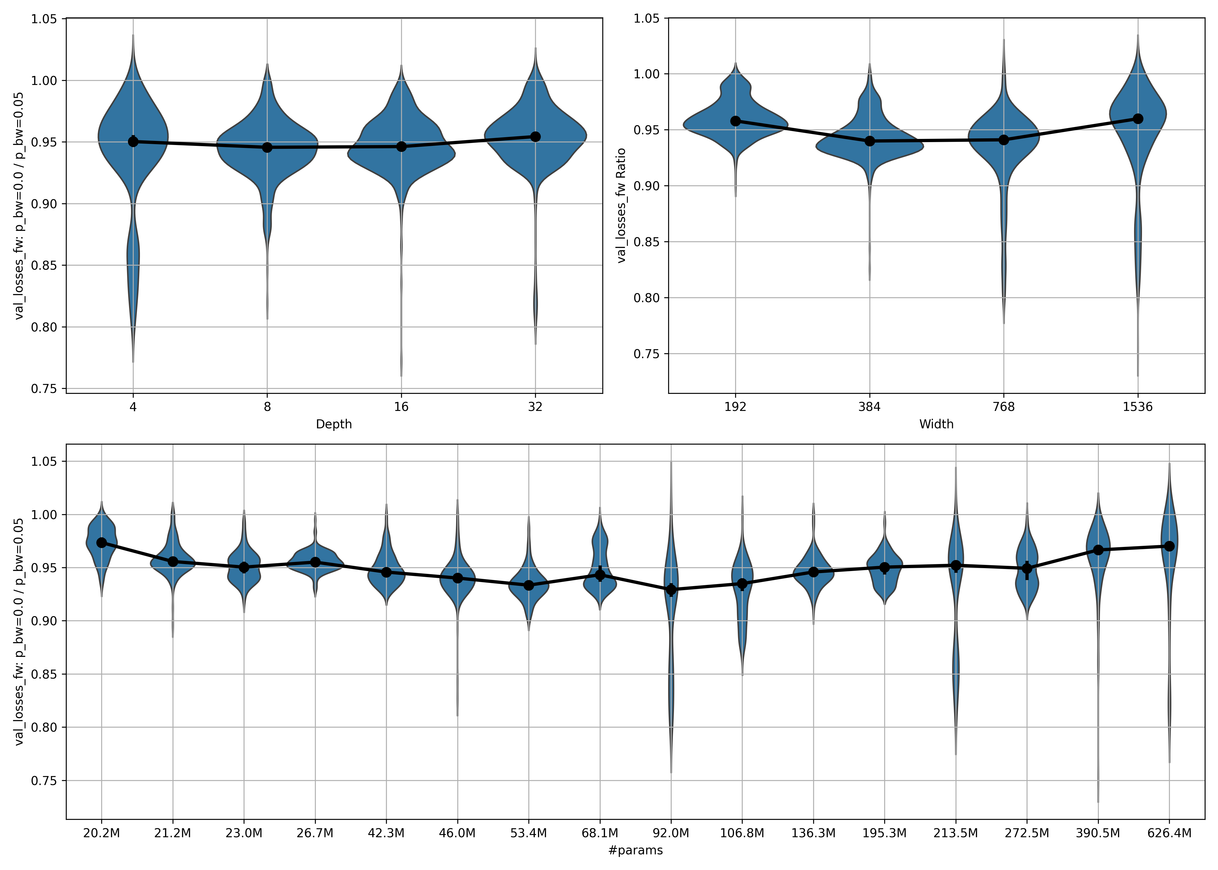
To check out how the performance looks after the models have been trained for a bit, let’s look at the ratio for epochs 5 to 10. This means that the poor performance at early training phases doesn’t impact the statistics, and we get a better idea of what the models will converge to. Here is ($\mathrm{epoch}{\mathrm{start}} = 5, \mathrm{epoch}{\mathrm{stop}} = 10$)

Observations:

• The scaling effects are much stronger here!
• In the largest model, the median ratio is essentially 1.

Taken together, this makes me think that with more scaling, models trained with $p_{bw} = 5\%$ could have the same or even better fw performance as ones trained with $p_{bw} = 0\%$. I am, however, not sure if this is the case in general, or only for when training for many epochs.

Performance by model layer

Let’s cut away the model’s layers one by one and evaluate every time.

Ratio 1: $p_{bw} = 0\%$ / $p_{bw} = 5\%$; fw task

How does the relative performance of the models trained with $p_{bw} = 0\%$ vs those trained with $p_{bw} = 5\%$ change over the layers?

Note that I only compare the performance of the final checkpoint here, so this is much less statistically meaningful than the analysis above, where I compared performance for many steps throughout training. However, it gives an indication of the trends in the models per layer and model size.

Because the differences in performance are so low, they are often rounded to $1.0$, which can give a wrong impression. So instead of the validation loss, I will plot the validation perplexity.

Let’s begin with ratio_then_mean, plotting ratio 1 over the number of layers remaining:

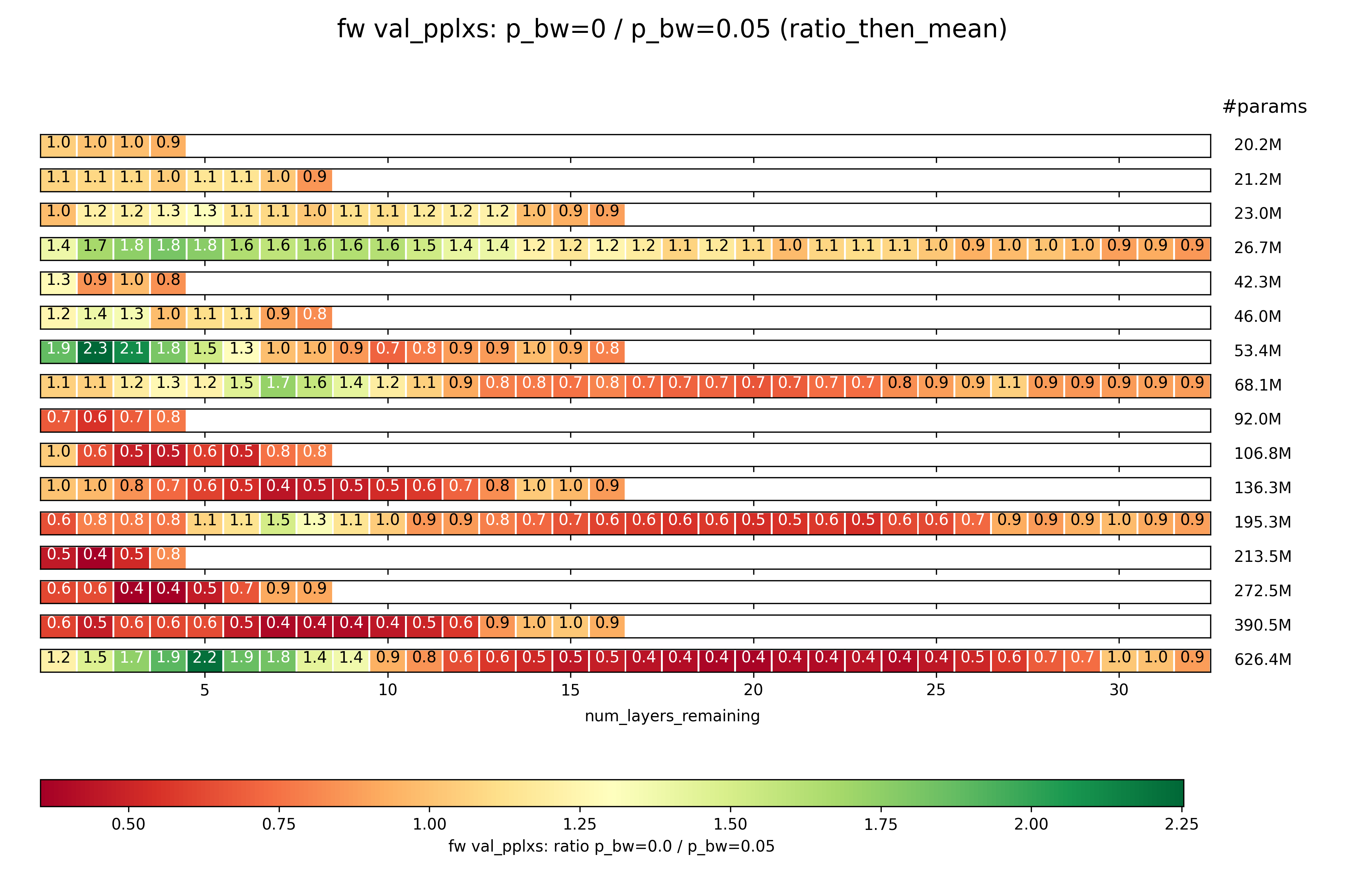
Some intersting things are going on here:

• In the deep models, it seems like the ratio is high in early layers. This means that early layers of models trained with $p_{bw} = 5\%$ are stronger in the fw task than those of ones trained with $p_{bw} = 0\%$.
• In the same deep models, the middle layers are awful for $p_{bw} = 5\%$ compared to the same layers for $p_{bw} = 0\%$.
• Only in late layers does the ratio recover and approach $1$ again.
• This could imply one of two things (or both at once, of course):
  1. Models trained with $p_{bw} = 0\%$ do a bunch of irrelevant stuff in early layers, do the real work in the middle layers, and then only refine somewhat in the late layers. Models trained with $p_{bw} = 5\%$ on the other hand show a more constant improvement in performance.
  2. Models trained with $p_{bw} = 5\%$ are forced to do a lot of good work in early layers, then take the bw task into consideration in the middle layers, and consolidate in late layers. Models trained with $p_{bw} = 0\%$ on the other hand show a more constant improvement in performance.

  It might be interesting to merge models trained with $p_{bw} = 0\%$ with ones trained with $p_{bw} = 5\%$.

And here is mean_then_ratio:

As you can see, this is identical, which indicates that there are no serious outliers in either the performance of $p_{bw} = 0\%$ runs or of $p_{bw} = 5\%$ runs.

Ratio 2: fw / bw task; $p_{bw} = 5\%$

How does the relative performance between the fw and bw task change? Importantly, this is not a comparison of fw performance for two different values of $p_{bw}$ as before, but a comparison between fw and bw performance for the same value of $p_{bw} = 5\%$.

Beginning with ratio_then_mean:

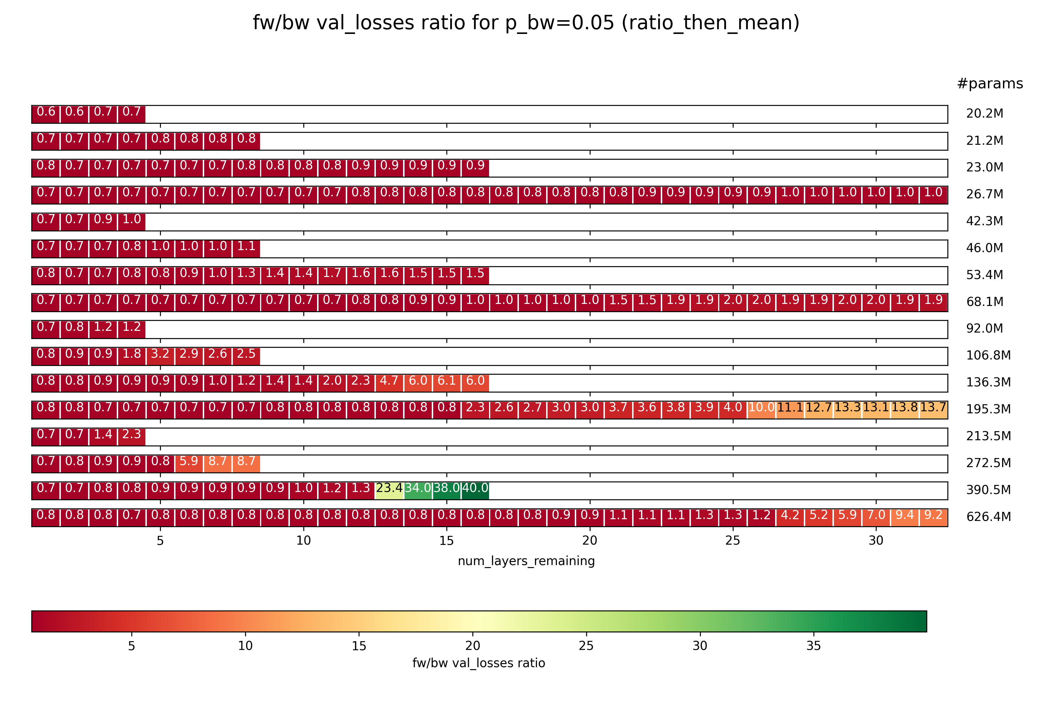
A few observations:

• As the number of layers is cut more and more, the performance of the bw task compared to the fw task drops off rapidly. This implies to me that the model learns the fw task, and performs that in the early layers, and then somehow manages to invert it into the bw task in the later layers.
• This transformation tends to go pretty slowly through most layers, and then suddenly jump.

To be clear, the absolute performance on both the fw and the bw task falls rapidly with every layer that is removed. However, as a trend, the later layers seem more important for the bw task, and the earlier layers for the fw task.

Now let’s look at the same thing, but calculated as mean_then_ratio:

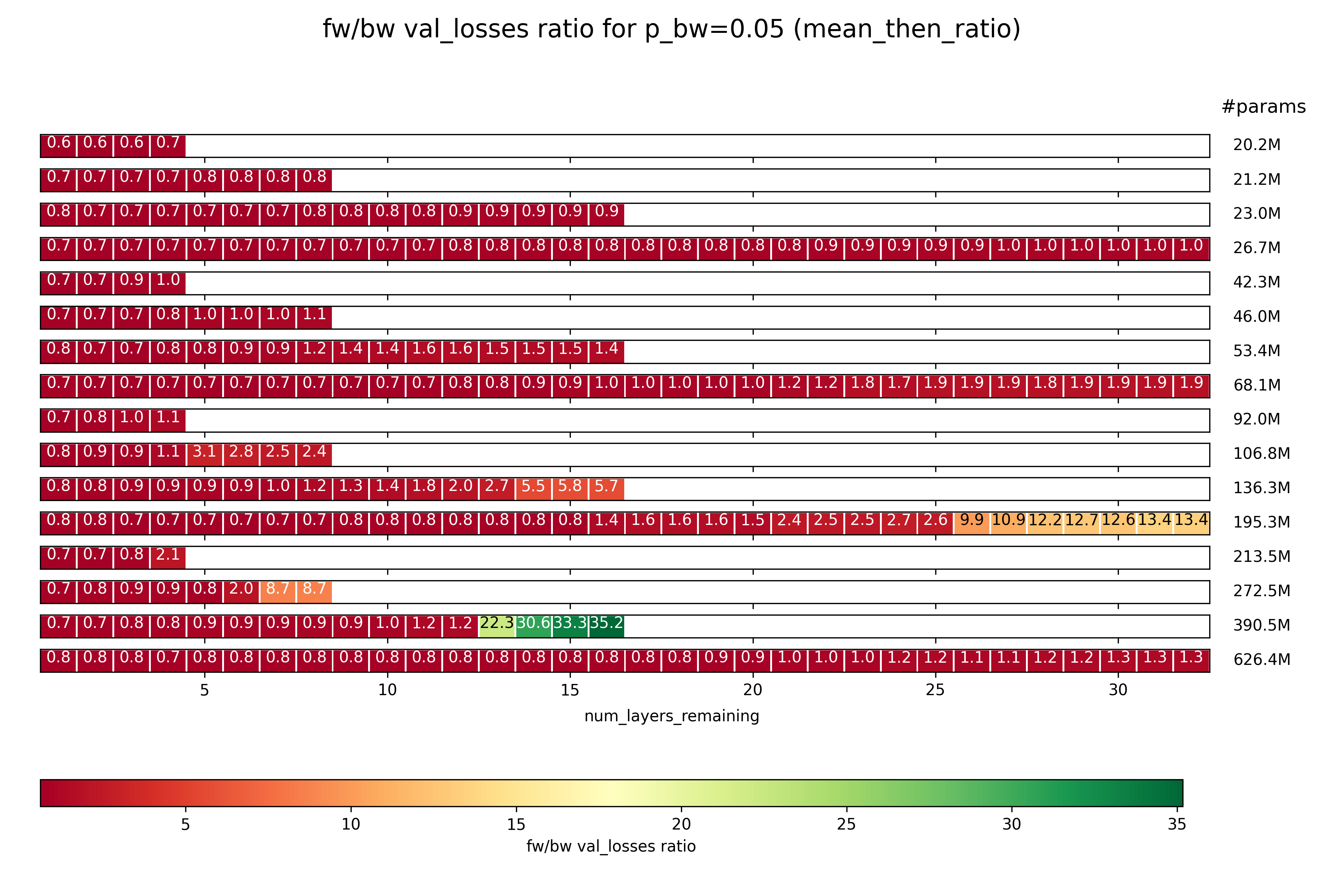
The same trend as above holds, but to a less extreme degree. That means that the variance in results is pretty high.

Future experiments

• Train on a larger dataset to see if we actually get a positive effect on the fw performance from training bidirectionally in one epoch, or if we need to train for multiple epochs.
• Instead of the choice being between training on either both the fw and bw task or only the fw task, make it a choice between training on just the fw or just the bw task.
• Finetune some open LLM on a dataset with this method, then train it to perform as a ColBERT-replacement RAG tool.

Acknowledgements

The code is modified from Fern’s hlb-gpt.

cff-version: 1.2.0
message: "Citations would be appreciated if you end up using this tool! I currently go by Fern, no last name given."
authors:
  given-names: "Fern"
title: "hlb-gpt"
version: 0.4.0
date-released: 2023-03-05
url: "https://github.com/tysam-code/hlb-gpt"

If you for some reason want to cite this work, here is the BibTeX entry:

@misc{snimu2024fwbwprediction,
  title={Forward-Backward Prediction},
  author={Sebastian Nicolas Muller},
  year={2024},
  month={5},
  url={https://github.com/snimu/https://github.com/snimu/blog/blob/main/contents/fw-bw-prediction/article.md}
}