The modded-nanogpt medium-track makes use of multiple tricks to improve performance, which rely on learned scalar values for mixing two vectors:
- U-Net: at three points in the model, the residual is modified by an earlier value of the residual via a weighted sum
- X0-Mixin: At every layer, after the U-Net skip (if it occurs at that layer) but before Attention and the MLP, the current residual and the original input embeddings are mixed in a weighted sum
- Value-Embeddings: In each Attention layer, value embeddings (extra embeddings of the input tokens) are added to the Value vector before the actual Attention operation is applied
I have measured and plotted the weights of these weighted sums; the lambdas. In this article, I will go through all three tricks, first explaining them shortly and then plotting the learned lambdas over the layers and training steps.
Warning: these are all from a single training run, so variations are possible.
This is for the code as of August 9th, 2025, corresponding to this record log. You can find the code here. If you have any feedback or ideas, I’d love to hear it on this Twitter post.
UPDATE 2025-08-12: I have unfortunately mixed up the labels of x_lambda and x0_lambda, which completely changes my analysis of the x0-lambdas section. I’m very sorry; I hate being a source of misinformation. The article has been updated: I have changed the x0 section completely, but only made small edits to the other two sections.
Expand this part to see the original article in full.
## U-Net Lambdas (Old) The model mixes the activations at position `a` into those at the later position `b` in the following way: `x_b = x_b + lambda_ab * x_a`. These U-Net lambdas shorten the gradient path from the output to the input (they are residual connections skipping multiple layers), and are initialized to 1.0, which means that the model is initialized to have a short effective depth (or more accurately, that the middle layers contribute fairly little). In a way, the value of the U-Net lambdas is a skip percentage. If a lambda is at 1, the layers that it crosses are skipped by 50%; if they are 0, they are skipped 0%. I'm sure that there are also different ways to look at these lambdas, but this is the most intuitive way to me. The following layers are connected: - 2 → 11 - 4 → 10 - 6 → 9 This makes for three scalar values that are optimized for the entire model. Here is their development over the course of training: 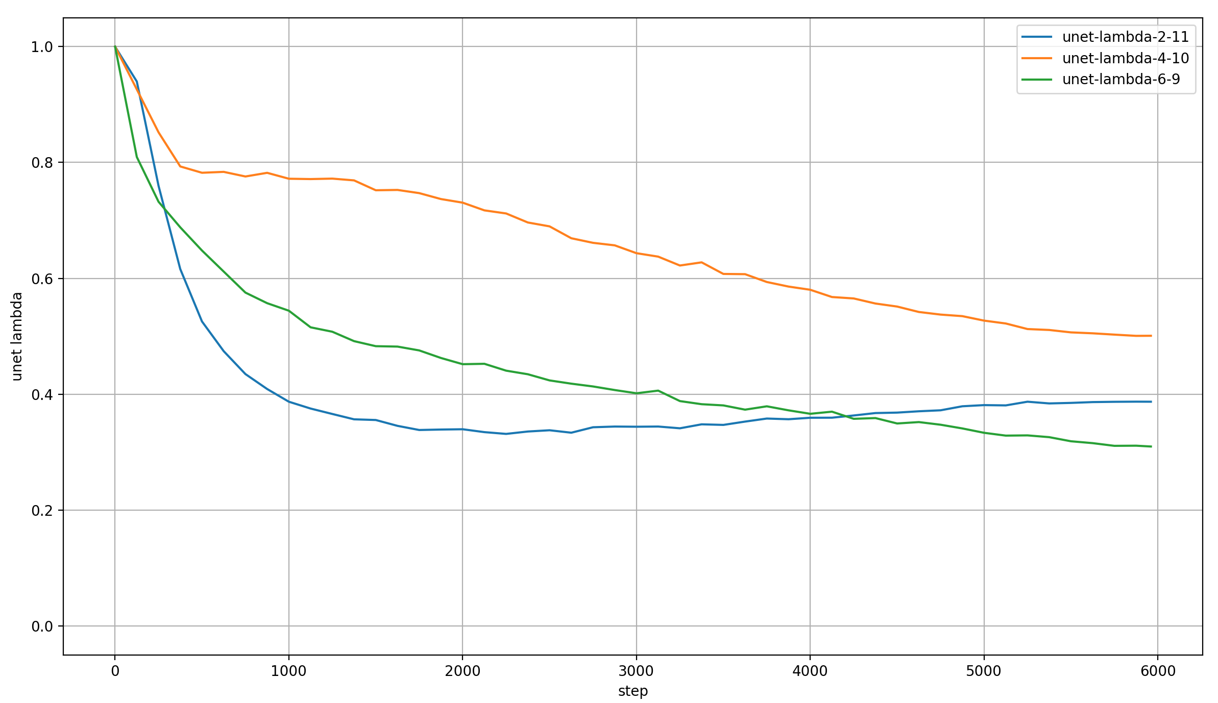 I find it interesting that the amount of layer-skipping at the end of training is still very significant: - Layers 0-2 and 11-15 are never skipped (by design) - Layers 3-10 are skipped via the 2-11 connection by ~0.4 / 2 → 20% - Nested within them, layers 5-9 are skipped via the 4-10 connection by 0.5 / 2 → 25% - And then among those, layers 7 and 8 are skipped via the 6-9 connection by ~0.3 / 2 → 15% The middle layers contribute relatively little to the output! Of course, that can be made up for by scaling the norm of the middle-layer outputs (which I unfortunately didn't measure), but my guess is that it's meaningful. ## X0-Lambdas (Old) At every layer of the model, there are two scalars used for mixing the input embeddings `x0` into the residual stream in a weighted sum: `x = x_lambda * x + x0_lambda * x0`. I don't fully understand the purpose of this modification to the standard transformer architecture. It definitely makes for a very short gradient path to the input, and also provides a gradient to the input embeddings from every layer, speeding up their training. In the backward pass, the layers effectively act as data augmentations to the gradient, which allows for longer training with the same data and will thus be helpful for updating the embeddings. But I feel like that's not the full story. Anyway, I have recorded the x0-lambdas for all layers over the entirety of training. Plotting all of these is very ugly, so for my main plot I only show the final value of the x0-lambdas over the model's layers, normed so that their absolute values sum to 1 (because we care about their relative weight): 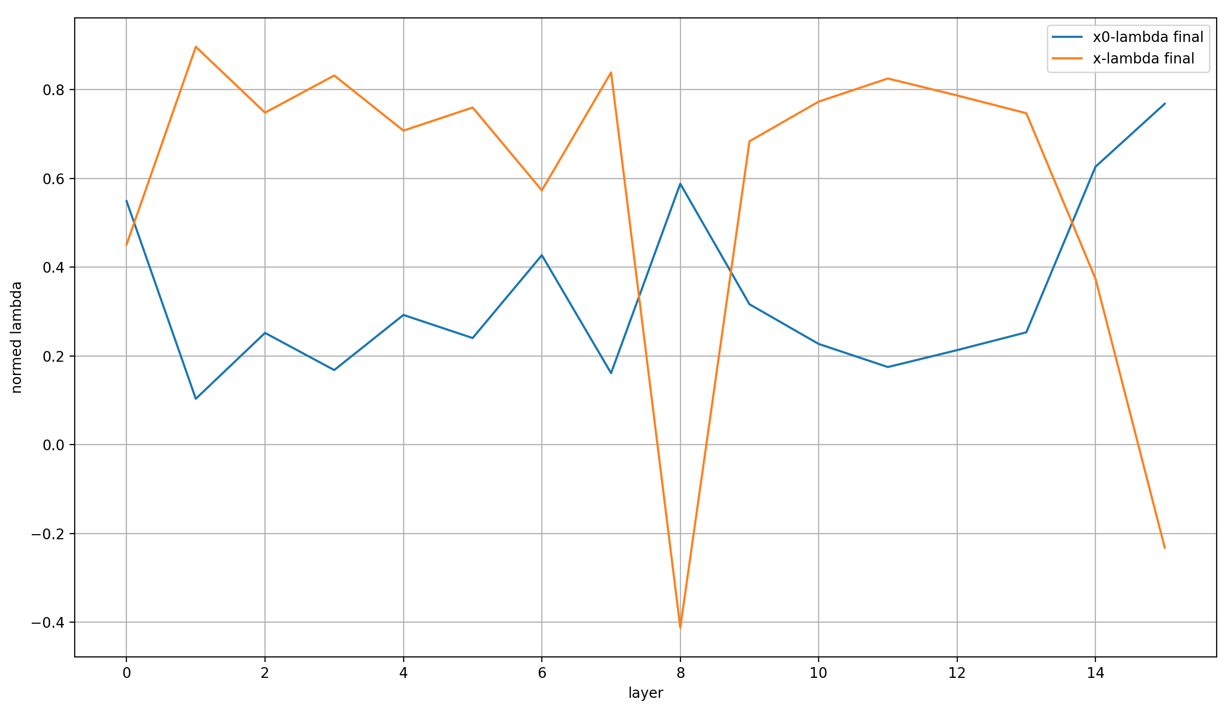 I can see three points of interest: First, the lambdas are almost identical in layer 0. That makes sense, because in layer 0 (and only in layer 0), `x == x0`. Secondly, at layer 8, the sign of the `x_lambda` is flipped. To reach this point, it has to cross 0! So at some point in training, layer 7 is almost completely ignored. Note the interaction with the U-Net lambdas: layers 7 and 8 are skipped pretty strongly anyway, so the previous layer contribute to the output even when the `x_lambda` is 0. Setting `x_lambda` to 0 at layer 8 does, however, set the contribution of layers 7 and 8 to zero and replacing them fully with x0, which apparently happens for a short time during training. What is also interesting is that the x0-lambda is noticeably higher in layer 8 than in the other layers (except for the last). That may be chance, but it may also be a result of a specific architectural decision: layer 7 doesn't contain an Attention layer, only the MLP. This weakly suggests that layer 7 contributes less to the model than the other layers, and is thus overwritten more strongly with x0 (which is supported both by the strong skipping of middle layers via the U-net lambdas, and by the setting to zero of the `x_lambda` at layer 8). Lastly, the last layer has a very large x0-lambda. Almost 80% of the input to layer 15 consists of the input embeddings (which is again achieved by the x-lambda crossing 0 and becoming negative). That makes me view the final calculation as a simple embeddings calculation, like the stereotypical "king - man + woman = queen"; the transformer simply calculates the difference between the input and target embeddings. That is a common view of transformers, but it's accentuated in modded-nanogpt. It also reveals a second purpose of the x0-lambdas: they allow the model to compare the residual—meaning, in abstract terms, the vector it plans to add to the input embeddings—to the input to which it will be added—so x0—and adjusting accordingly. That's a bit imprecise, but it helps my intuition. It reminds me of the [Hierarchical Reasoning Model](https://arxiv.org/abs/2506.21734), where (a function of) x0 is used at multiple points to guide the generations of the main model. --- Now, let's look at the x0-lambdas over the layers *and* over the course of training. First the normalized values: 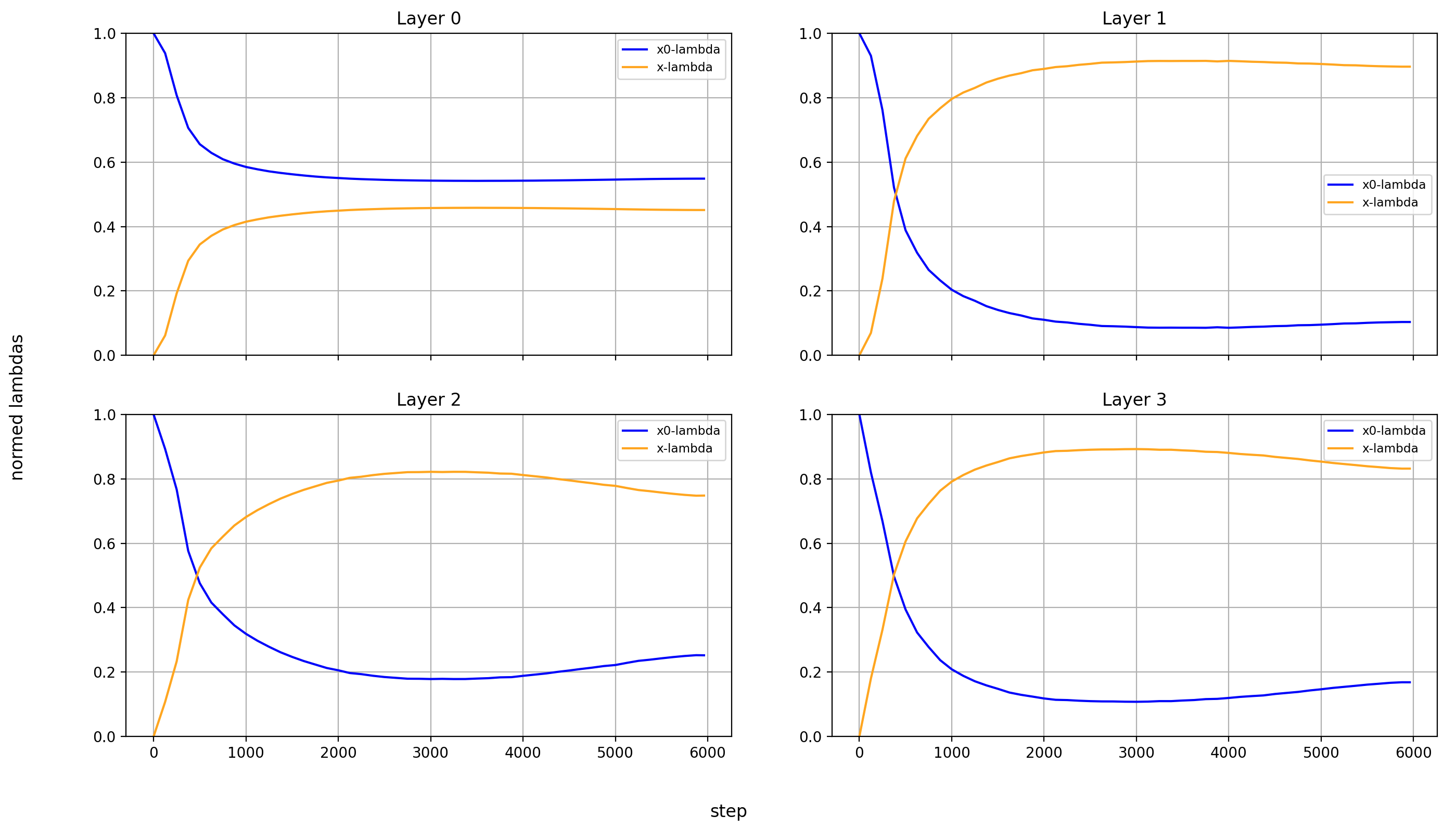 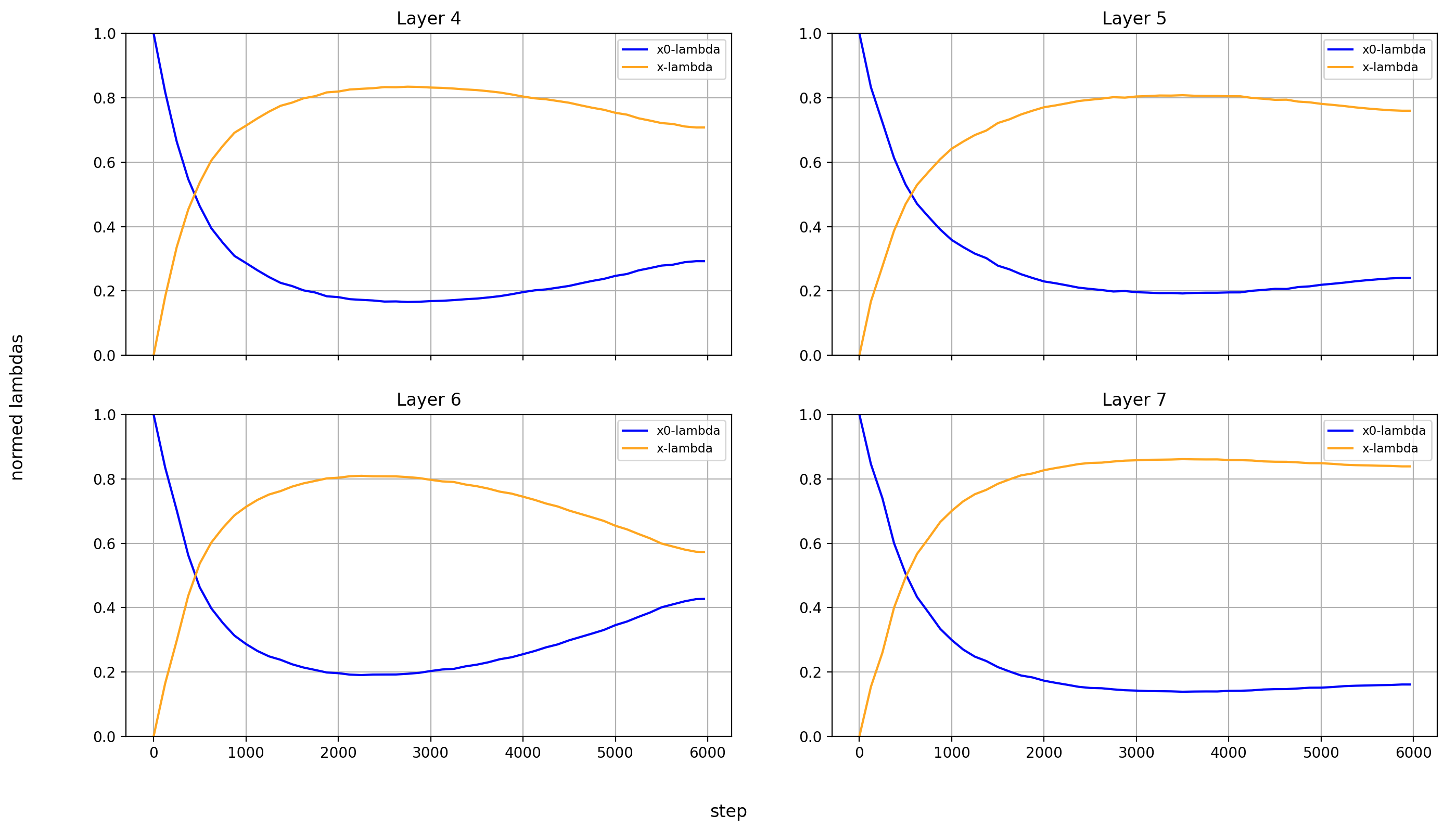 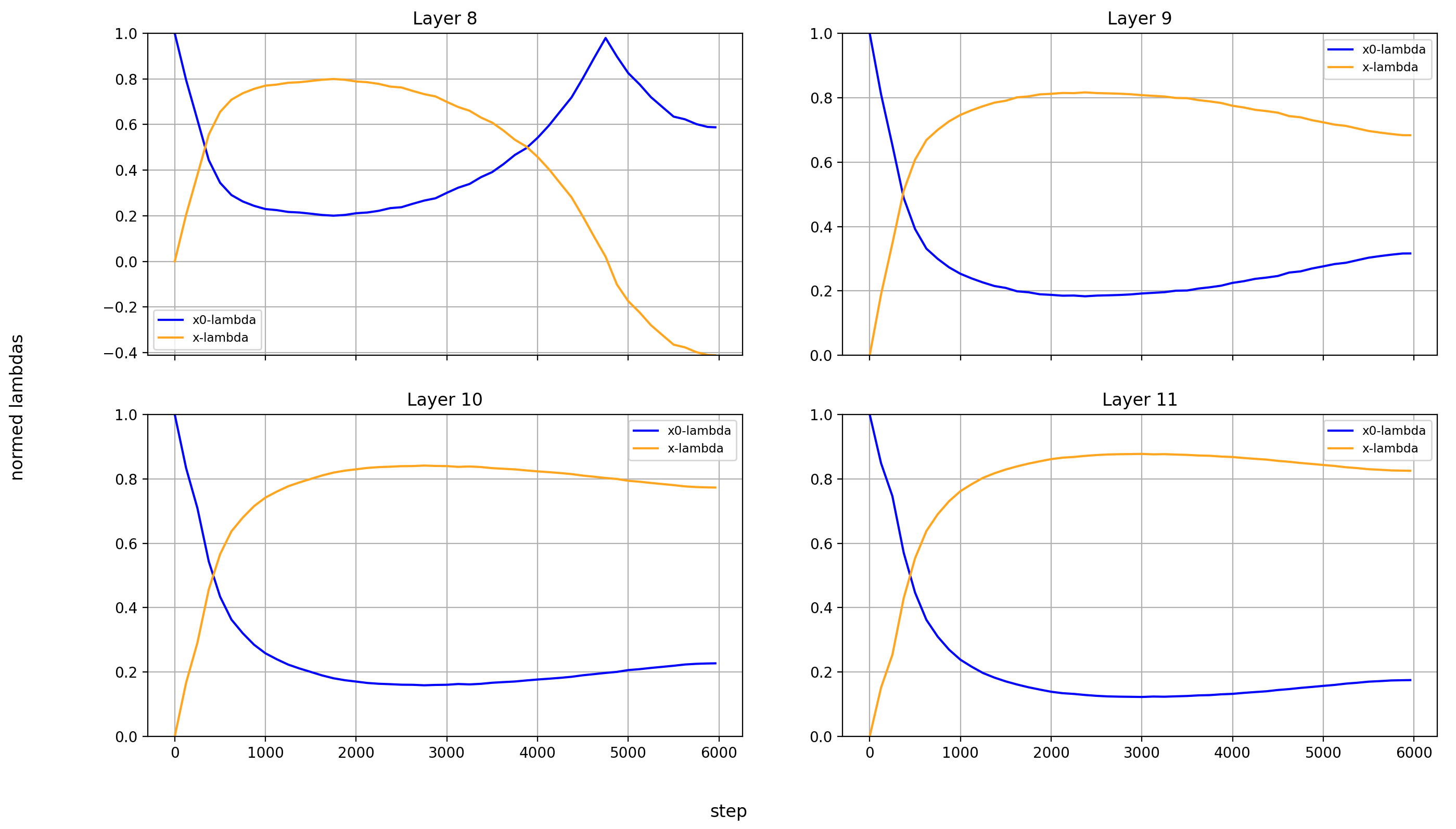 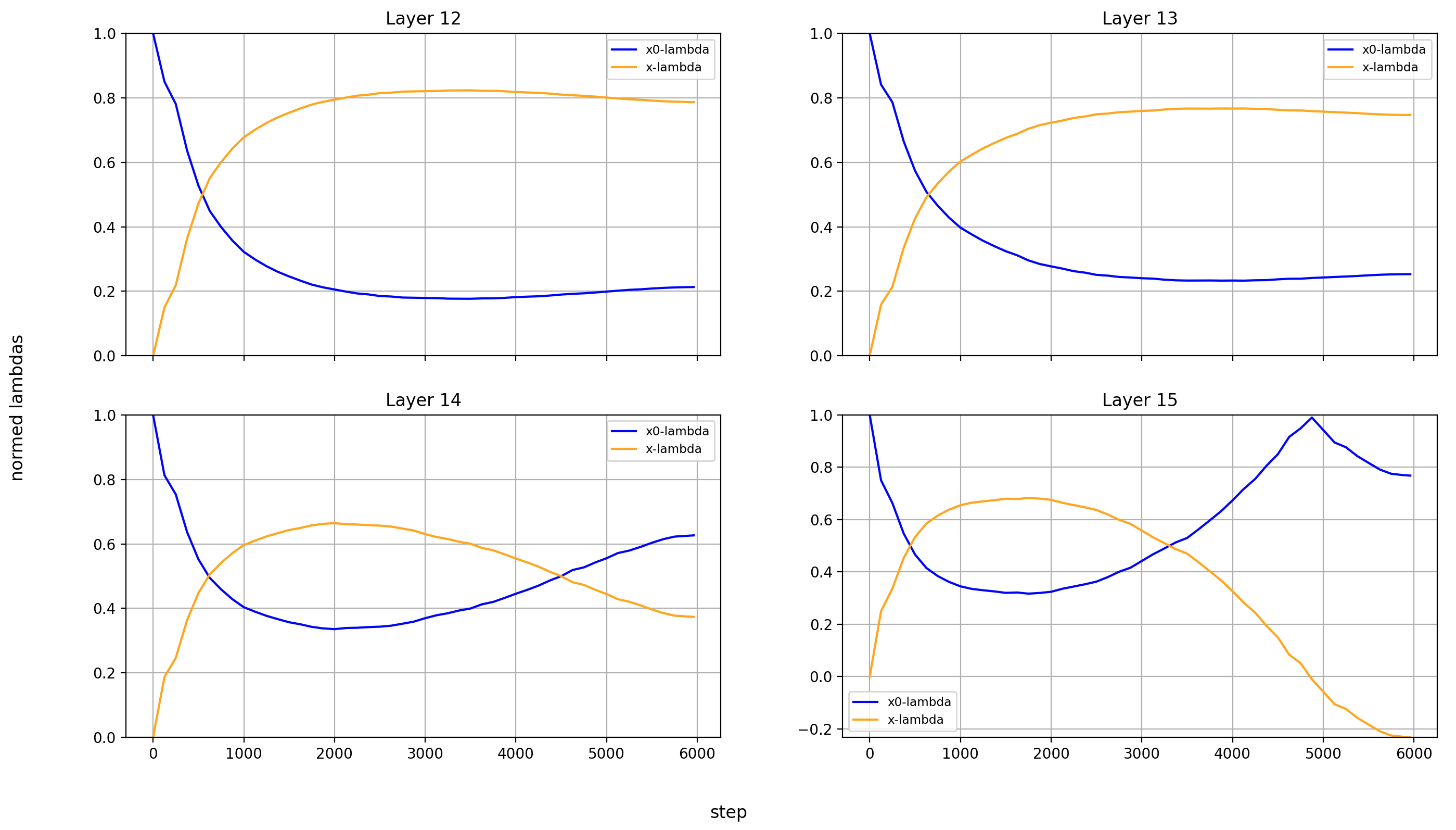 What immediately jumps out to me is that the lambdas develop very smoothly in all layers *except* in layers 8 and 15. But of course, this irregularity just comes from `x_lambda` crossing the 0-point. More interesting is that `x_lambda` first grows relative to `x0_lambda`, before dropping off a cliff and crossing over into negative territory. It's also curious to me that the crossover into negative values happens so late in training. In a static setting, I would say that inverting the sign of an activation isn't a huge deal, because this can be made up for with the weights. But in this case, the weights were adapted to a positive `x_lambda` most of the training run. In that case, inverting the sign *is* meaningful, and it reminds me of embeddings-math again. For this, it's also very important that both crossovers happen at the same time, so the two mostly make up for each other. The effects of the crossover of `x_lambda` to negative values are therefore threefold: 1. The interaction with x0 changes between layers 8 and 15 2. The interaction with the value embeddings (more on those [below](#value-embeddings-lambdas)) changes in layers 13 and 14 3. At layers 8 and 15, the impact of x falls to 0 and then rises again, meaning that for a short while, they produce their outputs only based on x0 (and the value embeddings in the case of layer 15) The last point is remarkable. Layer 15, which is the very last layer of the model, for a short while represents a single-layer transformer that takes to different embeddings of the same input tokens as its input. And this doesn't cause a spike in the validation loss: 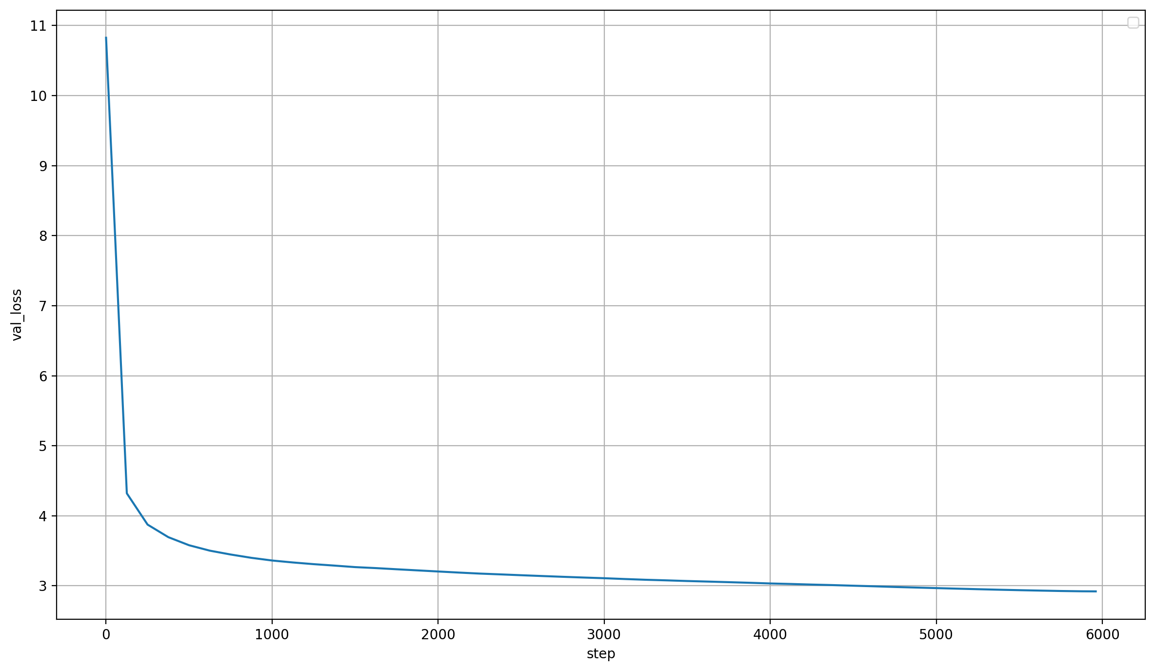 It's also noteable that layer 14 is the only other layer in which the impact of x0 exceeds the impact of x at the end of training. It's especially interesting because that's how it starts, but for a large part of the middle of training, the inverse is true. A third phenomenon is that the impact of x rises over most of training, and then falls again at the end, *in every single layer* but the first (where it doesn't matter). This tends to happen earlier than the crossover of `x_lambda` into negative values in layers 8 and 15. I wonder how these dynamics are connected to the learning rate schedule and the sequence length schedule (modded-nanogpt uses a block mask that increases in size over the course of training). So here is a plot of the learning rate and sequence length, relative to their absolute values (so normalized to between 0 and 1): 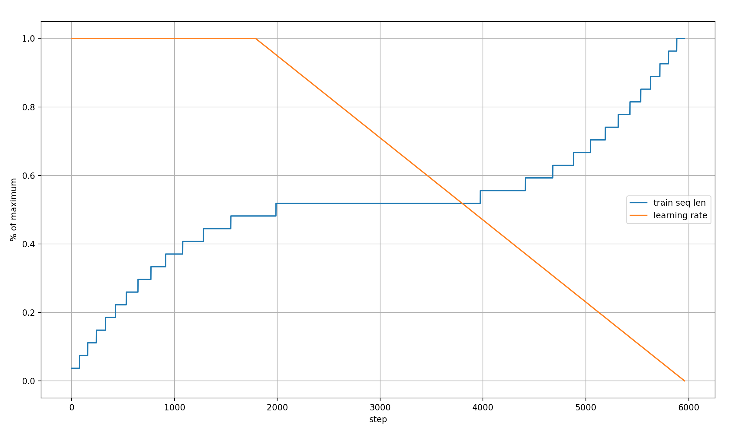 The learning rate is constant for the first ~2000 steps, then falls linearly to 0. The sequence length rises to half its maximum in the first ~2000 steps, then remains constant for ~2000 steps, before rising again in the last ~2000 steps. And that is indeed very informative! - The impact of x stops rising relative to x0 right around the time when the learning rate begins decaying, and the sequence length becomes constant - In layer 14, x0 becomes more important than x right after the sequence length begins increasing again - The `x_lambda` crossover happens shortly after that, which makes it look like it is also connected to the sequence length schedule Especially the second and third point are curious to me. Is the solution for dealing with sequence length extension to focus more strongly on x0? I don't know how meaningful these are, and how consistent they happen over different training runs, but the close relationship between hyperparameters and x0-lambdas make me think that there are real phenomena here. Now let's look at the absolute values: 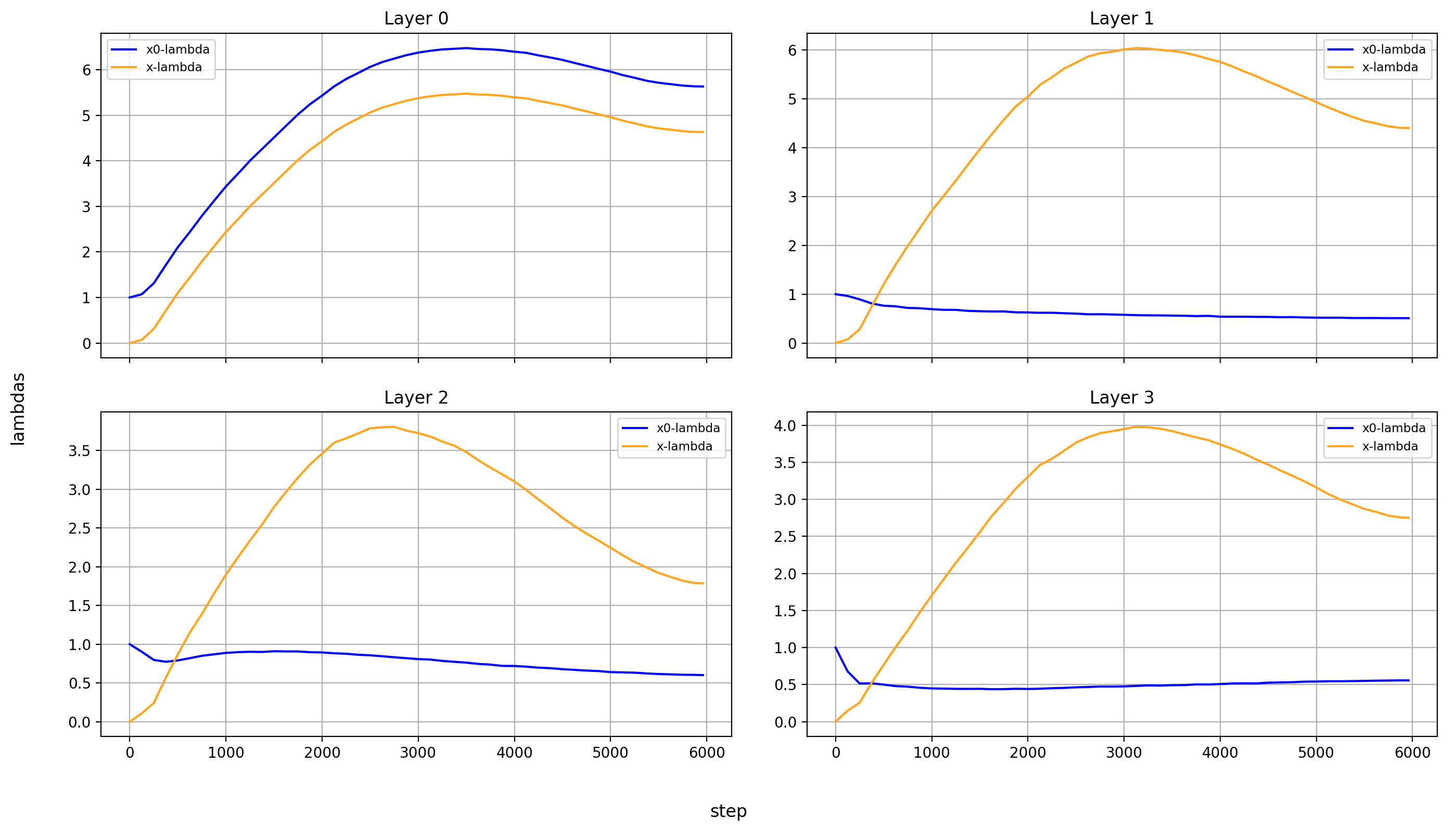 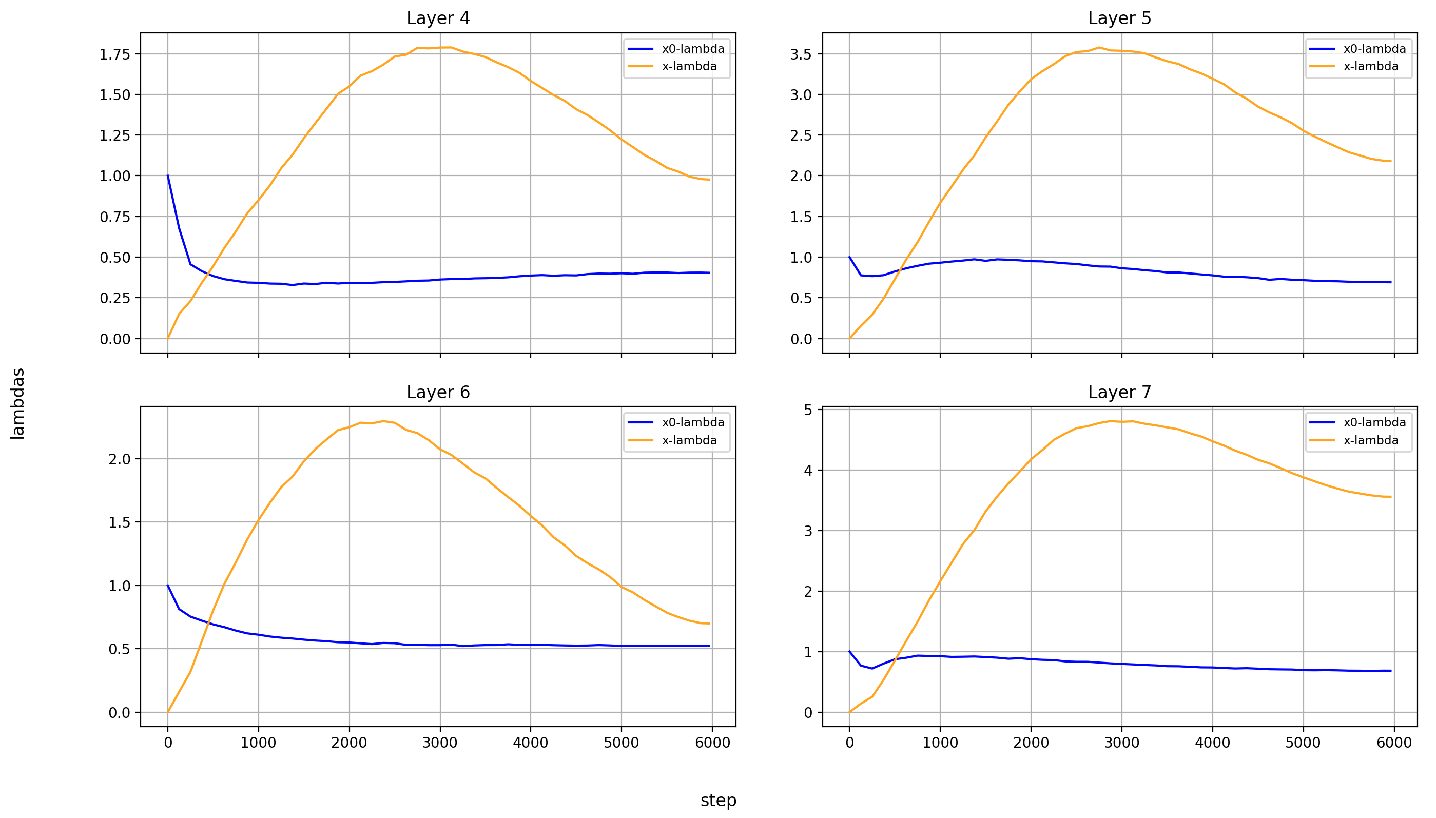 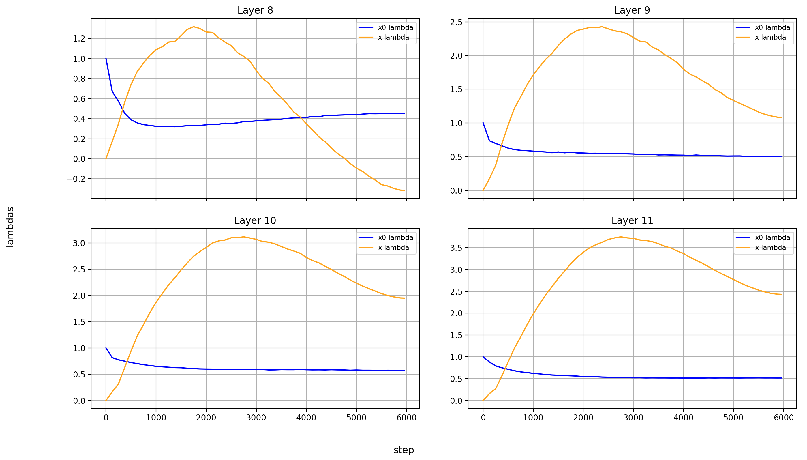 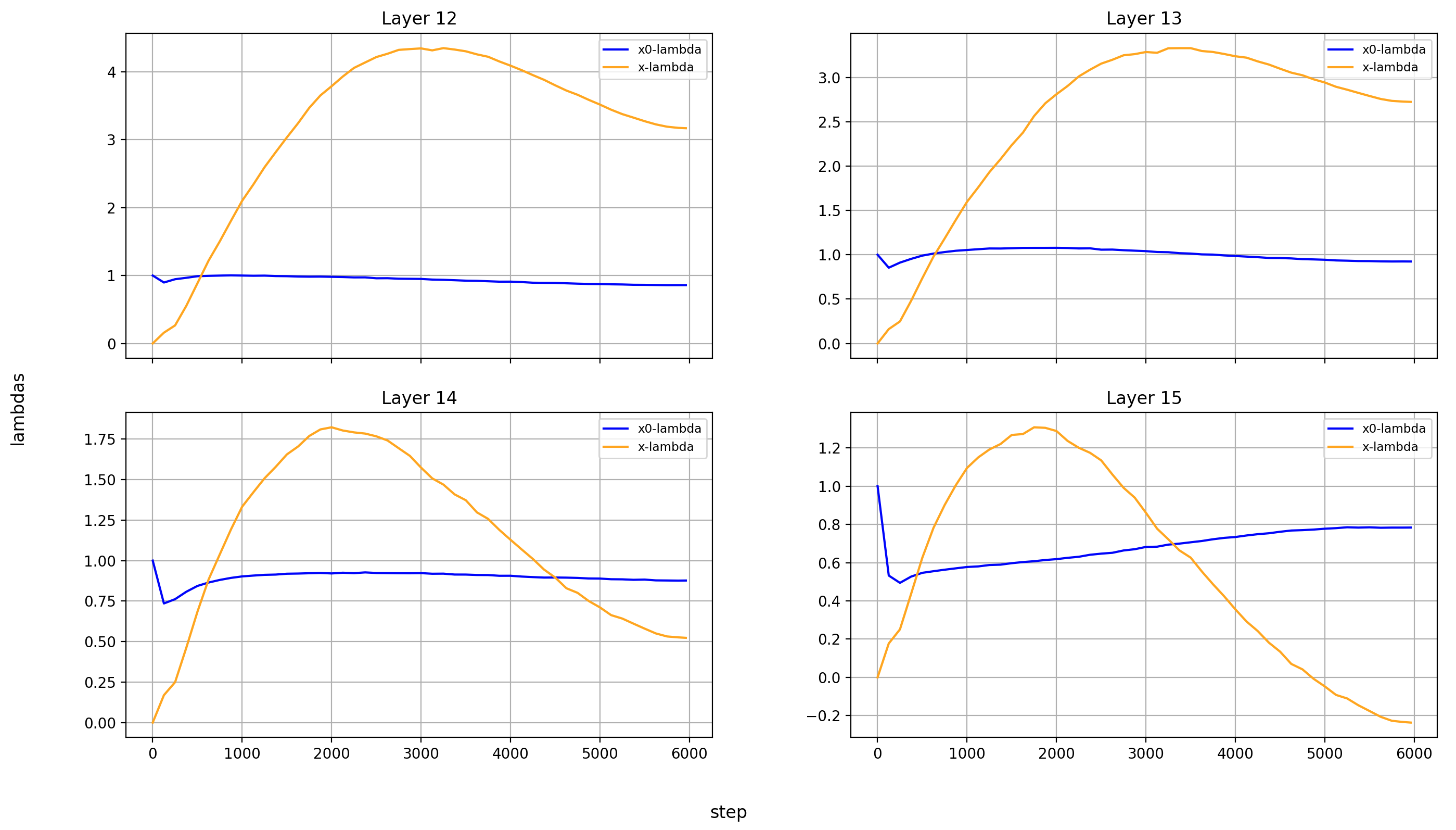 One interesting phenomenon is that the early layers tend to have higher absolute values than the later ones, so the impact of early layers is accentuated beyond the U-Net connections. Taking the U-Net connections into account, this means thats the effective model depth is shortened again, and middle layers add their algorithmic complexity in more subtle ways. But it might also be connected with the [value embeddings](#value-embeddings-lambdas), which are applied to the first and last three layers. High x- and x0-magnitudes in the first three layers suppress the relative impact of the value embeddings, while low magnitudes in the last layers will keep them high. But let's re-visit this later. Layers 8 and 15 are the layers with the lowest `x_lambda` and `x0_lambda`. I'm not sure what that means, just wanted to point it out. ## Value-Embeddings Lambdas (Old) The value embeddings are embedding layers beside the one that forms x0. Their embeddings are added to the Values in the causal self-attention block right before flexattention is applied: `v = v_lambda * v + ve_lambda * ve.view_as(v)` (where `ve` are the layer's value embeddings) However, that is only the case in the first and last three layers. In between, only `v_lambda` is used to scale the Values, while `ve_lambda` remains unchanged over training. And at layer 7, there is no attention, so there are no such lambdas. To add more complexity, the value embeddings of the first and last three layers are shared; so layers 0 and 13, layers 1 and 14, and layers 2 and 15 share the same value embeddings. This saves parameters and ensures that there is a short gradient path from the loss to the value embeddings. While additional gradient comes from the first three layers which are the farthest away from the input, there is always gradient from the three layers nearest to the loss, too. I admit that I only have some very weak intuitions for why value embeddings help. I've long held that token embeddings are a way to hold training-set wide statistics about the byte-sequence represented by the token, so I'm guessing that they add a way for the model to store more static per-token statistics which are helpful. Another viewpoint on this is that at least the value embeddings at the last three layers effectively reduce the model depth again. The most basic idea is that embeddings in general are a very cheap way to add parameters to an LLM (because they don't require a matrix multiplication, just a lookup) However, that's 100% speculation and you shouldn't take it too seriously. More importantly, I will again plot the final values of these lambdas over the layers. However, this time both the absolute and the relative values are of interest. The absolute values are specifically interesting for the layers in which there are no value-embeddings but `v_lambda` is still used to scale the values. The normed values are particularly interesting (at least in my eyes) for the layers where values embeddings are applied, because I'm interested in their weight relative to the values. So here is the plot with the absolute values: 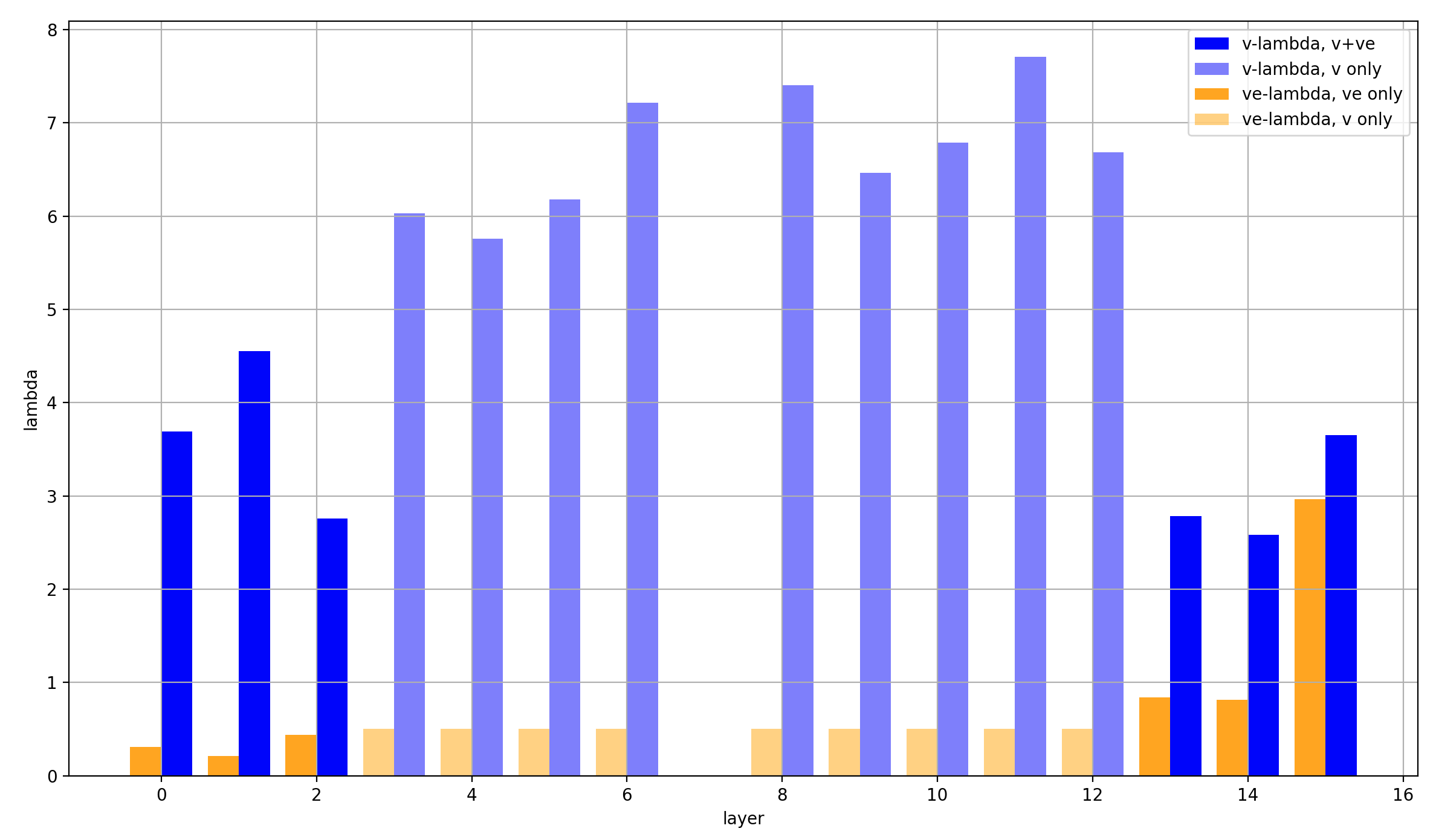 Some observations about the layers without value embeddings (layers 3-12): - The model really likes to scale the attention-values by around 6-7 via `v_lambda` - There seems to be a trend to do this more strongly in the later layers, but it's weak and I don't know if it's meaningful - At these layers, `ve_lambda` of course stays unchanged throughout training, because it's never used Some observations about the layer with value embeddings (layers 0-2 and 13-15): - `v_lambda` is significantly larger than at initialization for all layers, though not as much as without value embeddings - `ve_lambda` stays very low, except in the last layer - The ratio of `v_lambda` to `ve_lambda` is much higher in the first than the last layers; the value embeddings seem to have little impact on the first few layers (at least numerically, they could still stabilize training, or add just enough to make a difference, or whatever, but this only adds to the high magnitudes of x and x0 from the [x0-lambdas](#x0-lambdas)). To make more sense of that last point especially, let's look at the normalized lambdas: 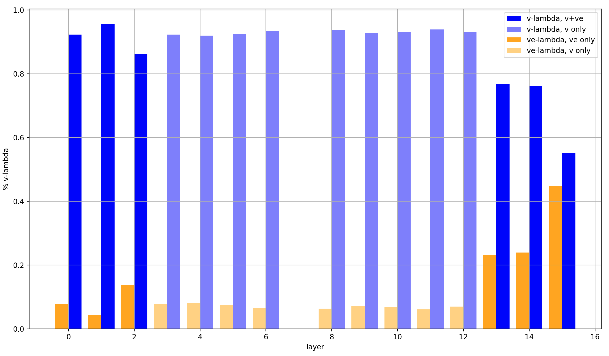 Three clear groups emerge: 1. Layers 0-2, which are affected very weakly by the value embeddings (by only around 10%) 2. Layers 13 and 14, which are affected fairly strongly by the value embeddings (by around 25%) 3. Layer 15, which uses its value embeddings almost as strongly as its input from the residual stream (with around 45% intensity) The last point is very interesting, because as we saw before, the last layer already mixes the original embeddings into the residual stream at its input with about 50% magnitude. That's a lot of fixed values that don't depend on the token-order at all! --- Let's look at the lambdas over the course of training again. First the normalized values: 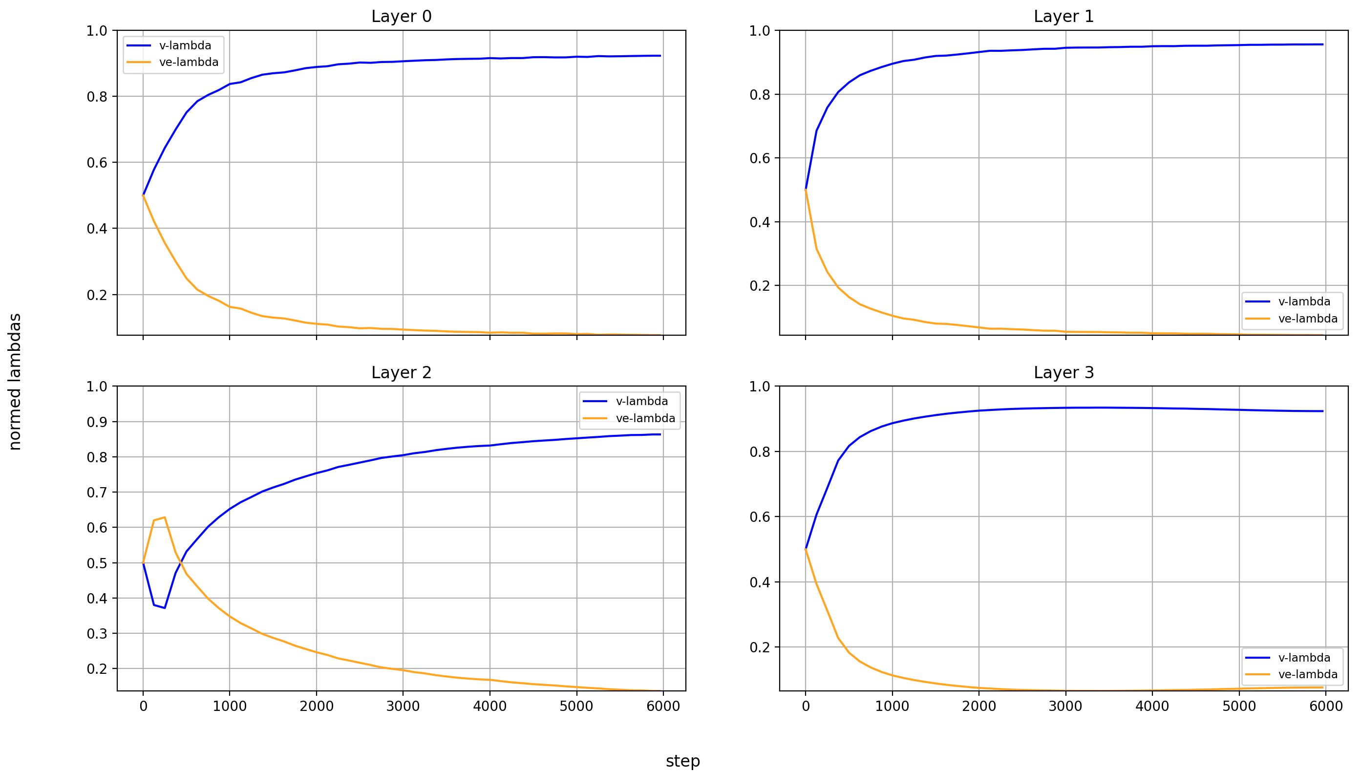 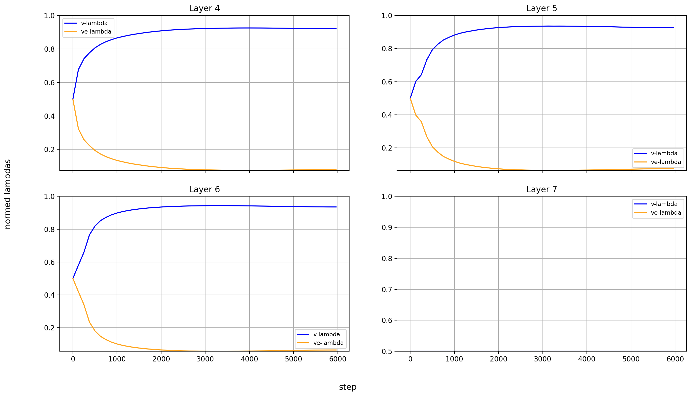 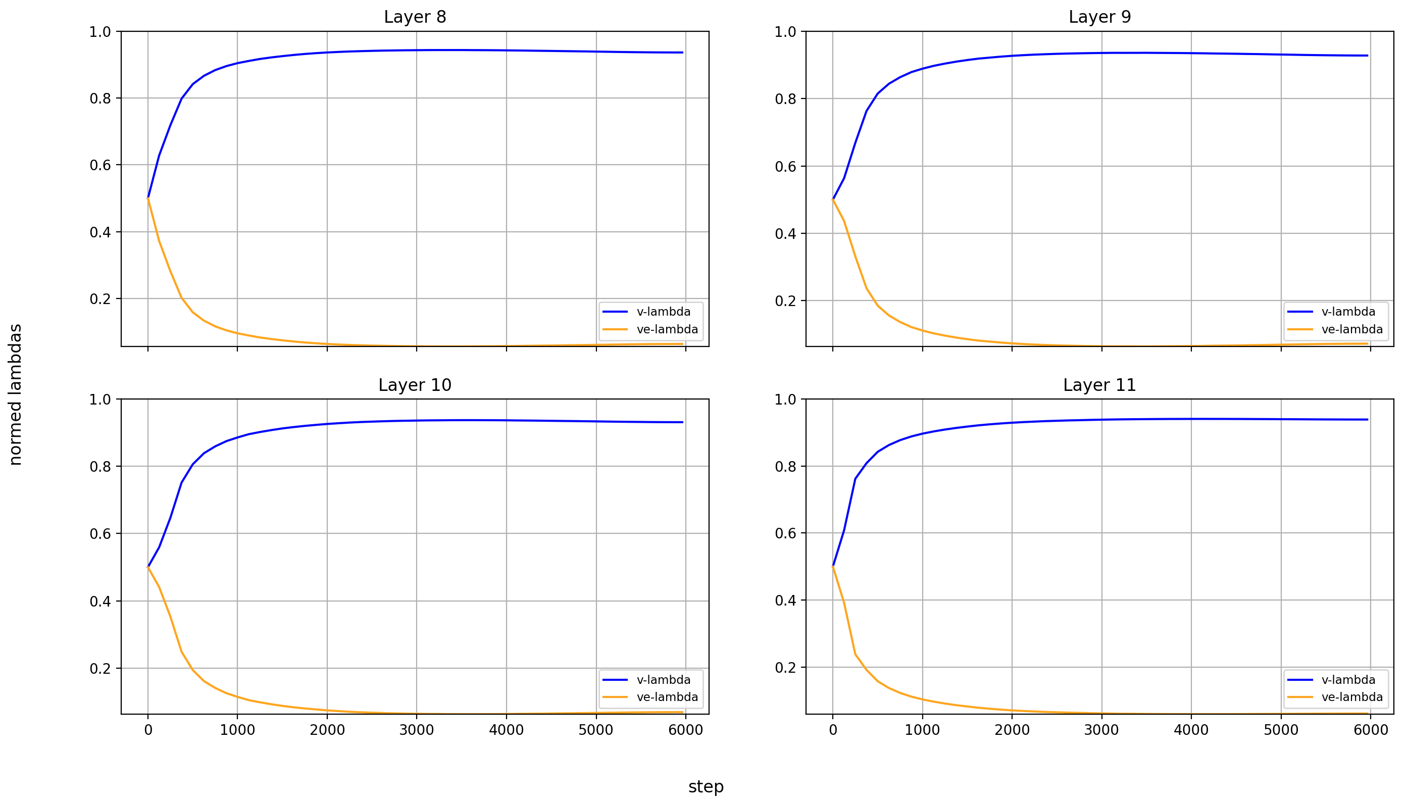 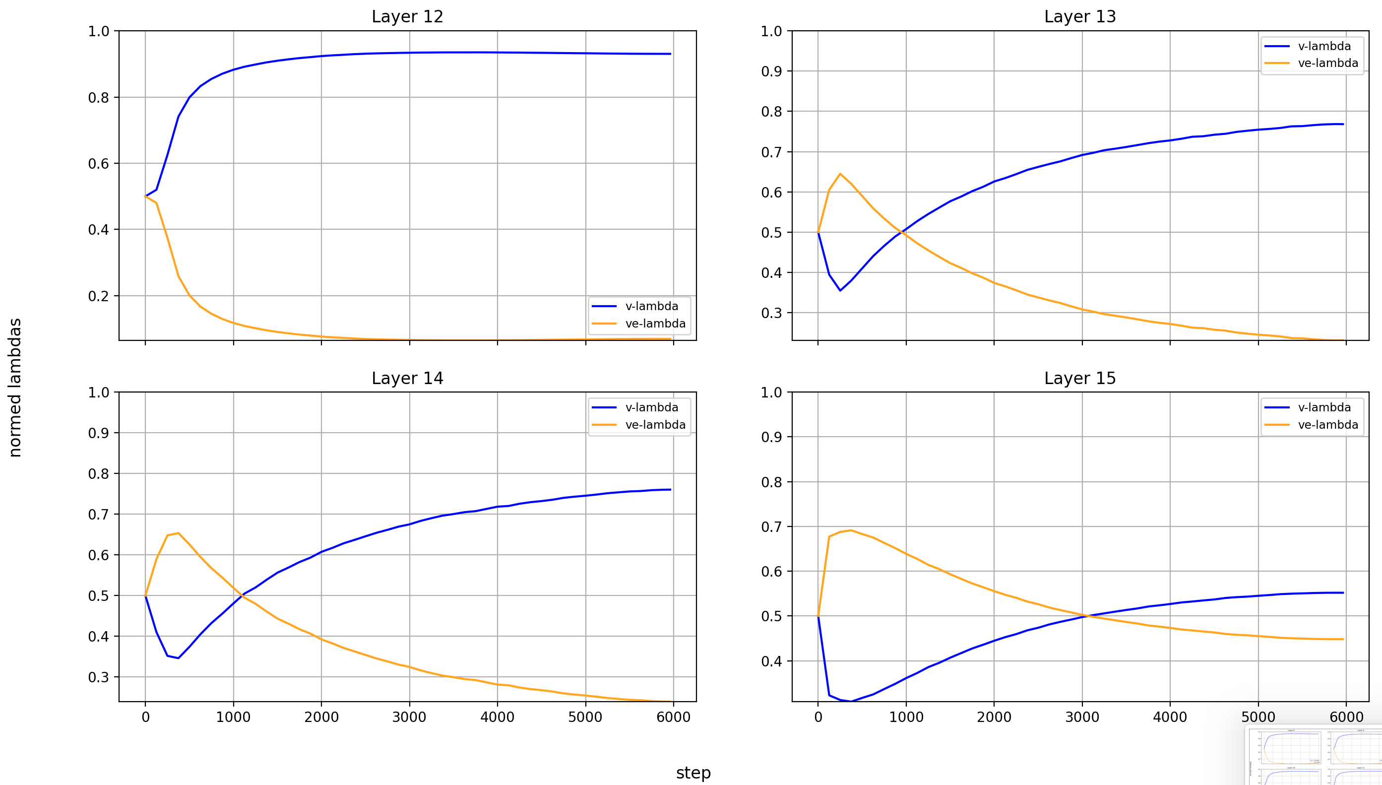 In the layers without value embeddings, the magnitude of the attention-values rises very quickly and never reverses course. But in the layer *with* value embeddings, only layers 0 and 1 behave similarly. For layers 2 and 13-15, the value embeddings first gain in relative importance before losing it again. The later the layer, the later this reversal happens. And here are the un-normed values: 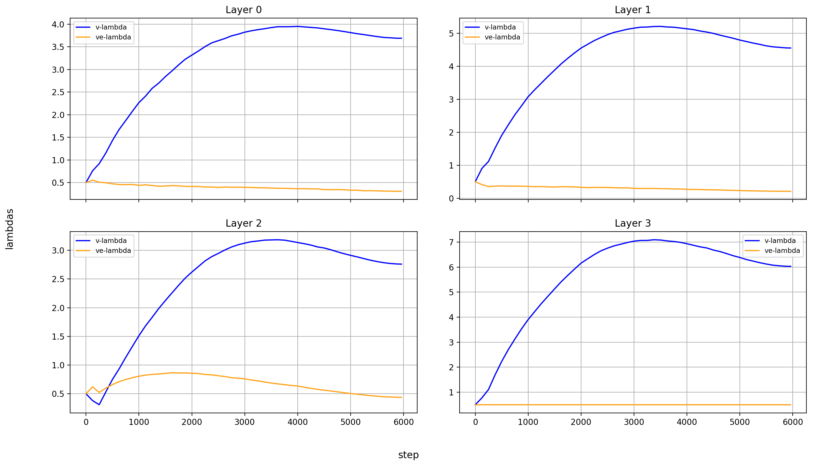 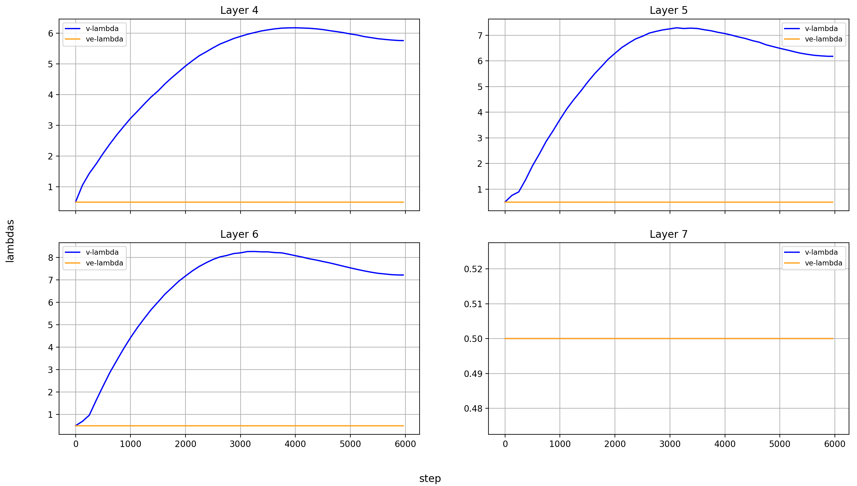 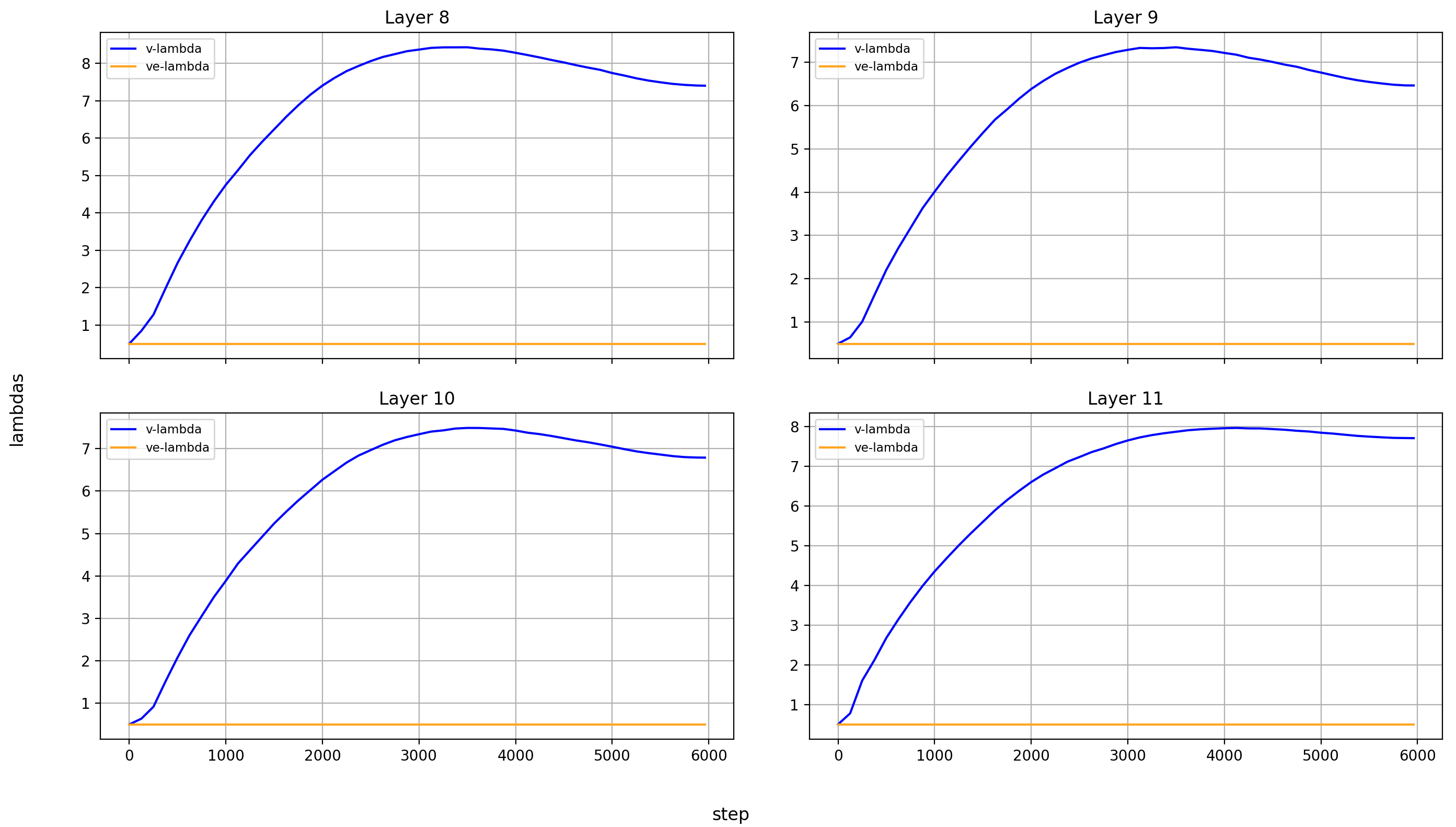 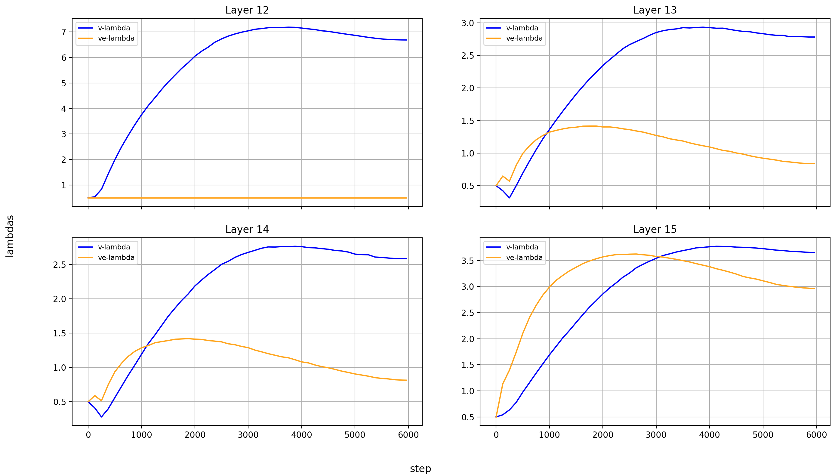 In all layers, the `v_lambdas` rise over most of training, before slightly falling toward the end. ## Summary I've ran the modded-nanogpt medium track training once (so don't overindex on this) and plotted all the scalar values that are being trained. Hope you enjoyed.U-Net Lambdas
The model mixes the activations at position a into those at the later position b in the following way: x_b = x_b + lambda_ab * x_a.
These U-Net lambdas shorten the gradient path from the output to the input (they are residual connections skipping multiple layers), and are initialized to 1.0, which means that the model is initialized to have a short effective depth (or more accurately, that the middle layers contribute fairly little).
In a way, the value of the U-Net lambdas is a skip percentage. If a lambda is at 1, the layers that it crosses are skipped by 50%; if they are 0, they are skipped 0%. I’m sure that there are also different ways to look at these lambdas, but this is the most intuitive way to me.
The following layers are connected:
- 2 → 11
- 4 → 10
- 6 → 9
This makes for three scalar values that are optimized for the entire model. Here is their development over the course of training:

I find it interesting that the amount of layer-skipping at the end of training is still very significant:
- Layers 0-2 and 11-15 are never skipped (by design)
- Layers 3-10 are skipped via the 2-11 connection by ~0.4 / 2 → 20%
- Nested within them, layers 5-9 are skipped via the 4-10 connection by 0.5 / 2 → 25%
- And then among those, layers 7 and 8 are skipped via the 6-9 connection by ~0.3 / 2 → 15%
The middle layers contribute relatively little to the output! Of course, that can be made up for by scaling the norm of the middle-layer outputs (which I unfortunately didn’t measure), but my guess is that it’s meaningful.
X0-Lambdas
At every layer of the model, there are two scalars used for mixing the input embeddings x0 into the residual stream in a weighted sum: x = x_lambda * x + x0_lambda * x0.
I don’t fully understand the purpose of this modification to the standard transformer architecture. It definitely makes for a very short gradient path to the input, and also provides a gradient to the input embeddings from every layer, speeding up their training. In the backward pass, the layers effectively act as data augmentations to the gradient, which allows for longer training with the same data and will thus be helpful for updating the embeddings. But I feel like that’s not the full story.
Anyway, I have recorded the x0-lambdas for all layers over the entirety of training. Plotting all of these is very ugly, so for my main plot I only show the final value of the x0-lambdas over the model’s layers, normed so that their absolute values sum to 1 (because we care about their relative weight):
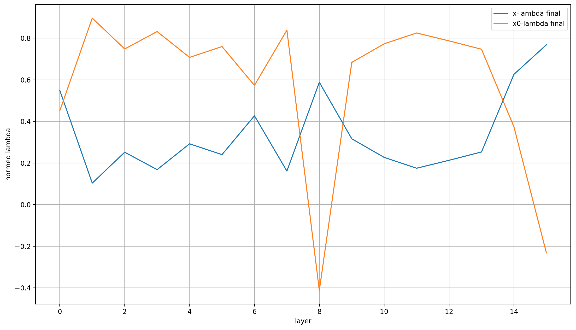
I can see three points of interest:
First, the lambdas are almost identical in layer 0. That makes sense, because in layer 0 (and only in layer 0), x == x0.
Secondly, x0_lambda is very high in all layers but three; higher than x_lambda in fact! This immediately reminds me of very simple embeddings math, like the classic “king - man + woman = queen” example. All the model does in the last layer is add a vector to the inputs to turn them into the outputs.
In this view, x0_lambda allows the model to compare the residual—meaning, in abstract terms, the vector it plans to add to the input embeddings—to the input to which it will be added—so x0—and adjusting accordingly. Throughout the model, x0_lambda dominates, so the model just continually refines the vector that it wants to add to x0 in the end, and the immediate view of x0 from x0_lambda allows it to correct course by comparing the output of the previous layer with the initial input.
That reminds me of the Hierarchical Reasoning Model, where (a function of) x0 is used at multiple points to guide the generations of the main model.
Thirdly, the last layers have an even higher x_lambda. In the view that I’ve just expressed above, I think it’s a useful simplification to view the model as just the last layer, which produces the final output by modifying the input x0. It does so via a learned bias in the form of the value embeddings which I’ll revisit below, and a dynamic compontent that is strongly influenced through guidance from the previous layers. So layers 0-14 calculate the direction of the vector update, and layer 15 applies the update (after small corrections) together with a bias to the input.
In reality, layer 14 already has a high x_lambda, so this view isn’t totally accurate; and of course in DeepLearning things are never that easily interpretable. However, I think that the evidence points to this view at least not being too far off, and it’s a nice intuition for me.
Lastly, it’s also interesting is that x_lambda is noticeably higher in layer 8 than in the other layers (except for the last two). That may be chance, but it may also be a result of a specific architectural decision: layer 7 doesn’t contain an Attention layer, only the MLP.
Since an MLP is essentially an embedding layer that happens to return a weighted sum of features instead of an individual feature per token, this MLP conceivably fulfill a bit more of the purpose of x0 already. That’s because while the tokens at its inputs are mixed, they probably aren’t perfectly mixed, and so the input token at each position will tend to dominate. Therefore, this layer acts a bit like a value embedding layer, but fully in the path of the residual.
And we should remember that the layer is skipped fairly strongly, which means that at layer 9 it’s outputs (as filtered through layer 8) are just mixed into the residual from layer 6, making it behave even more closely like a value embedding.
I need to stress that this entire third point is purely speculation, except for the statement of fact at its beginning.
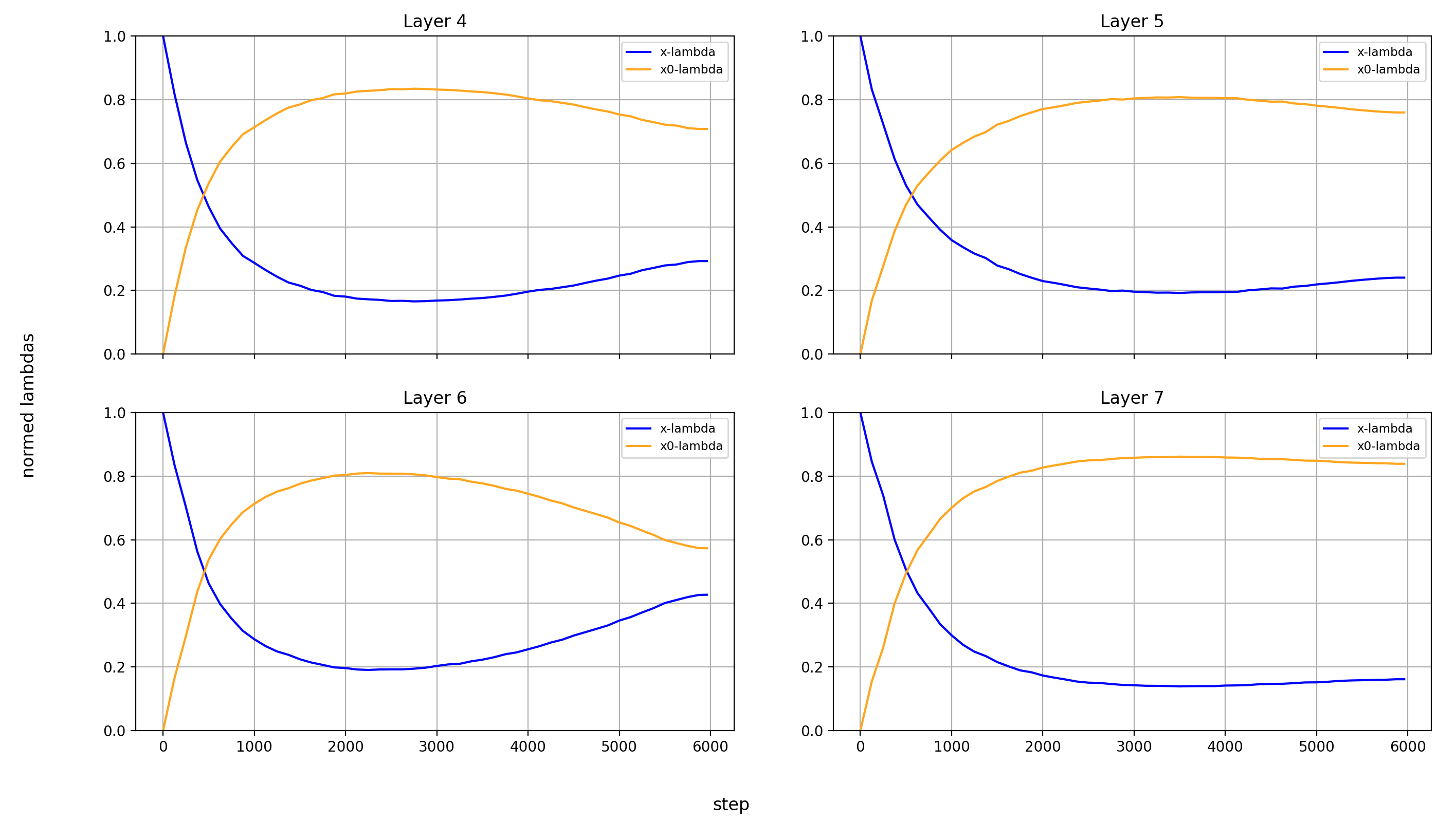
Now, let’s look at the x0-lambdas over the layers and over the course of training.
First the absolute values (because they show more interesting results):
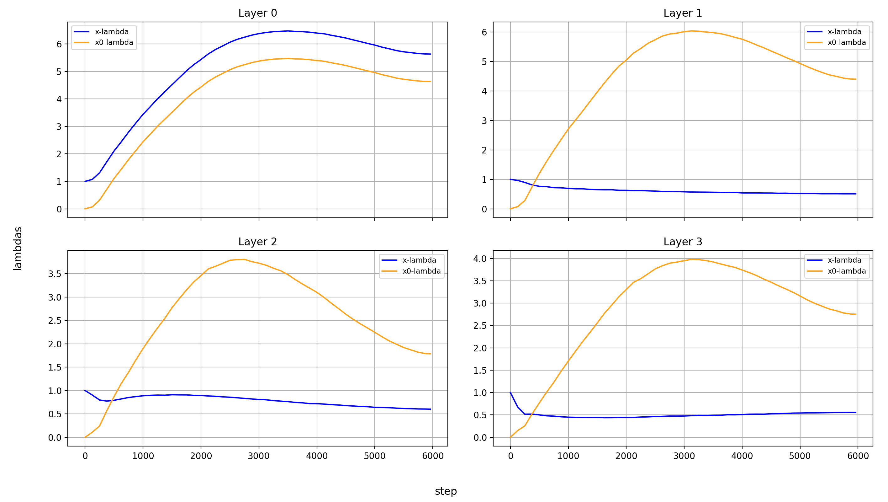
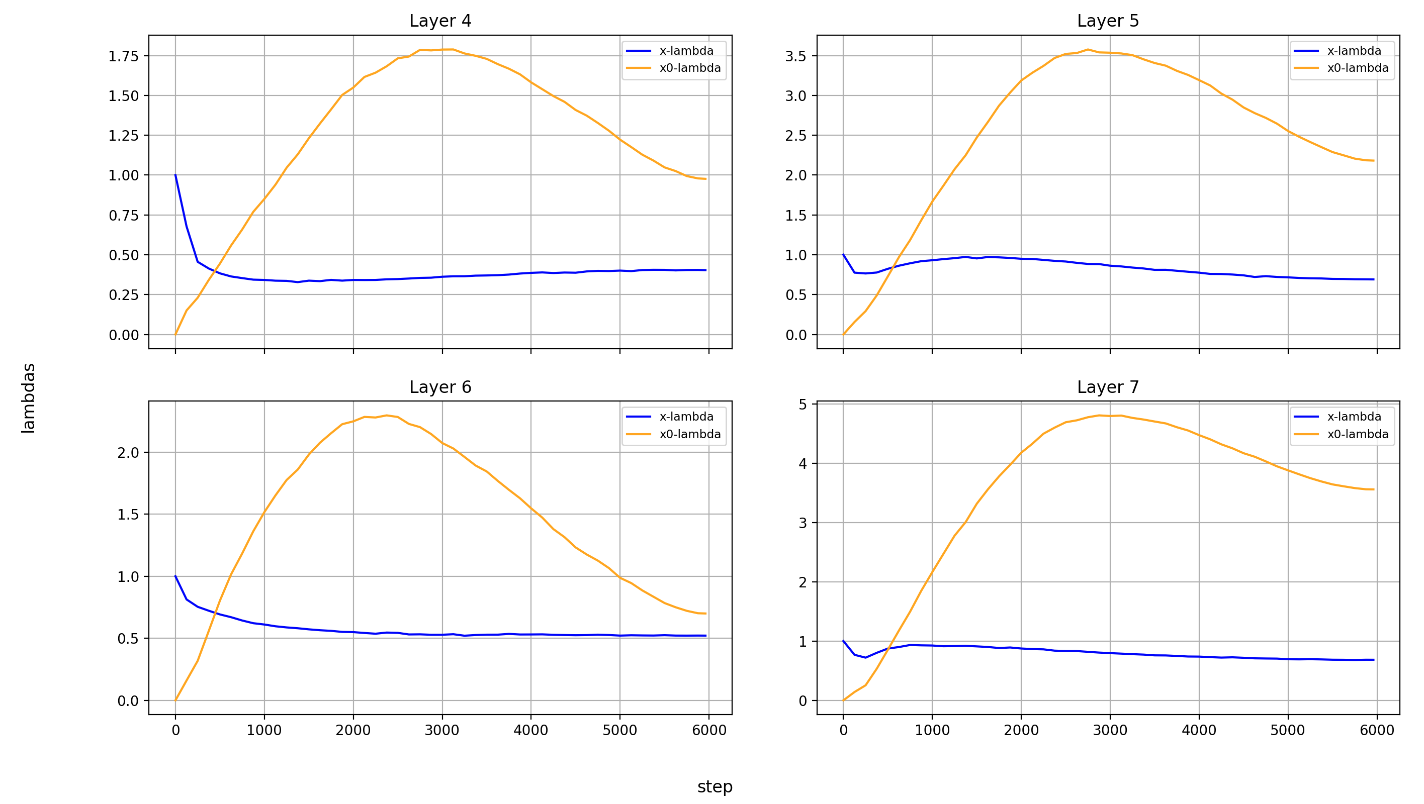
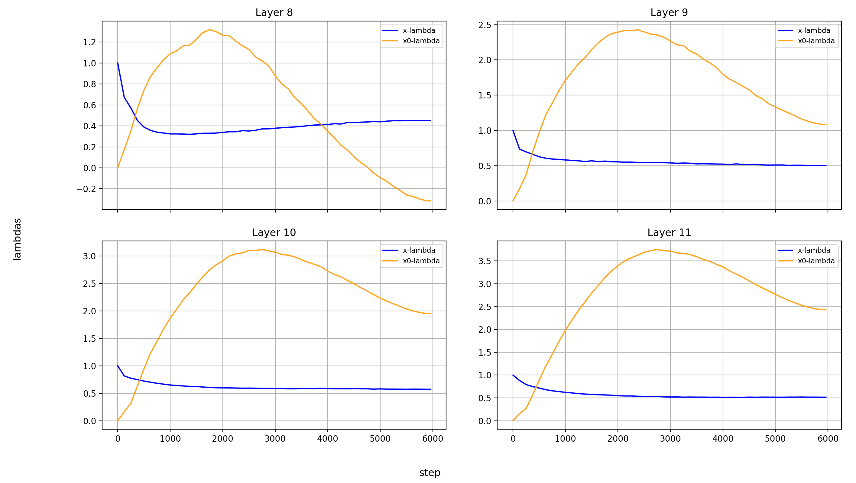
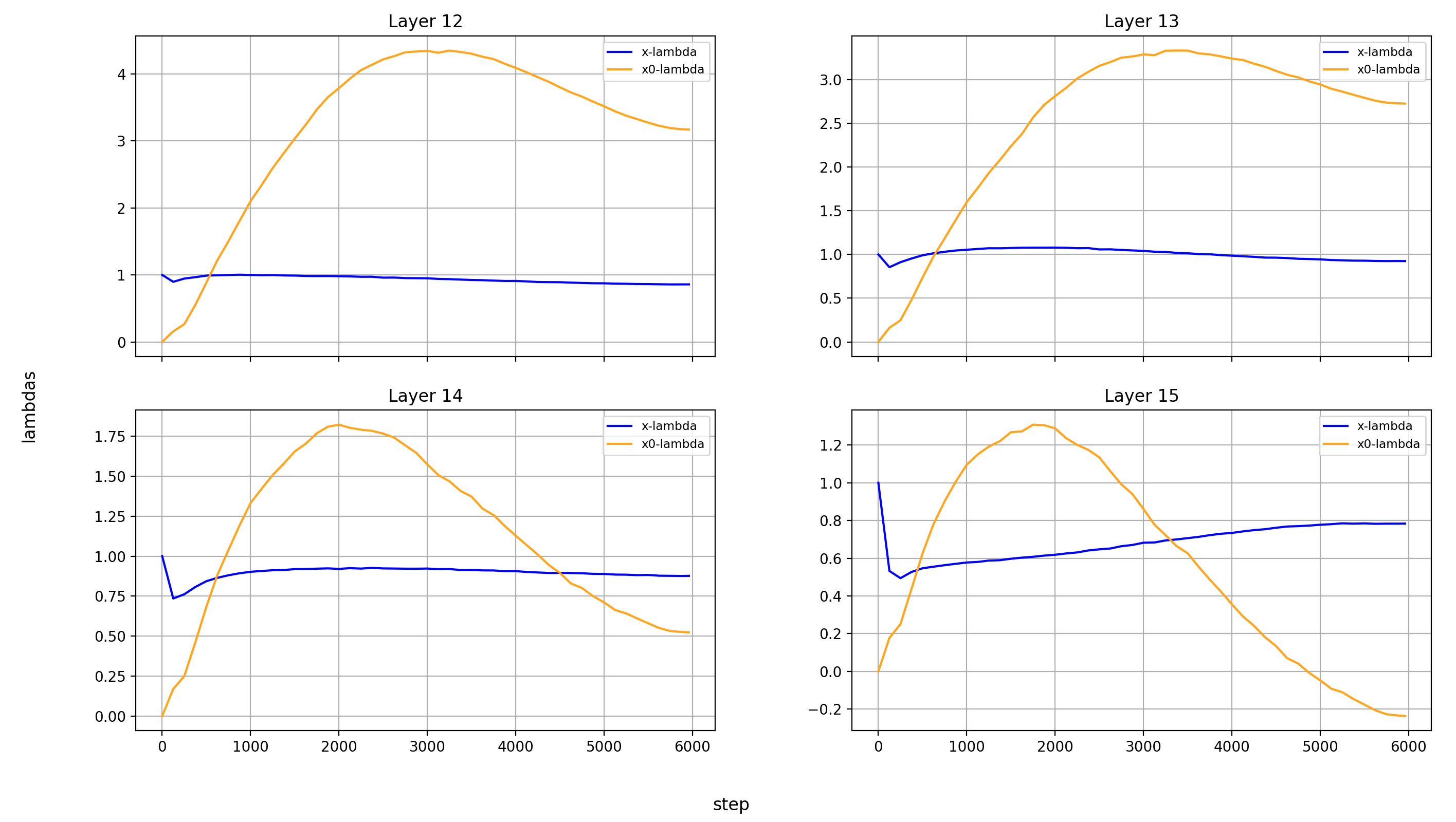
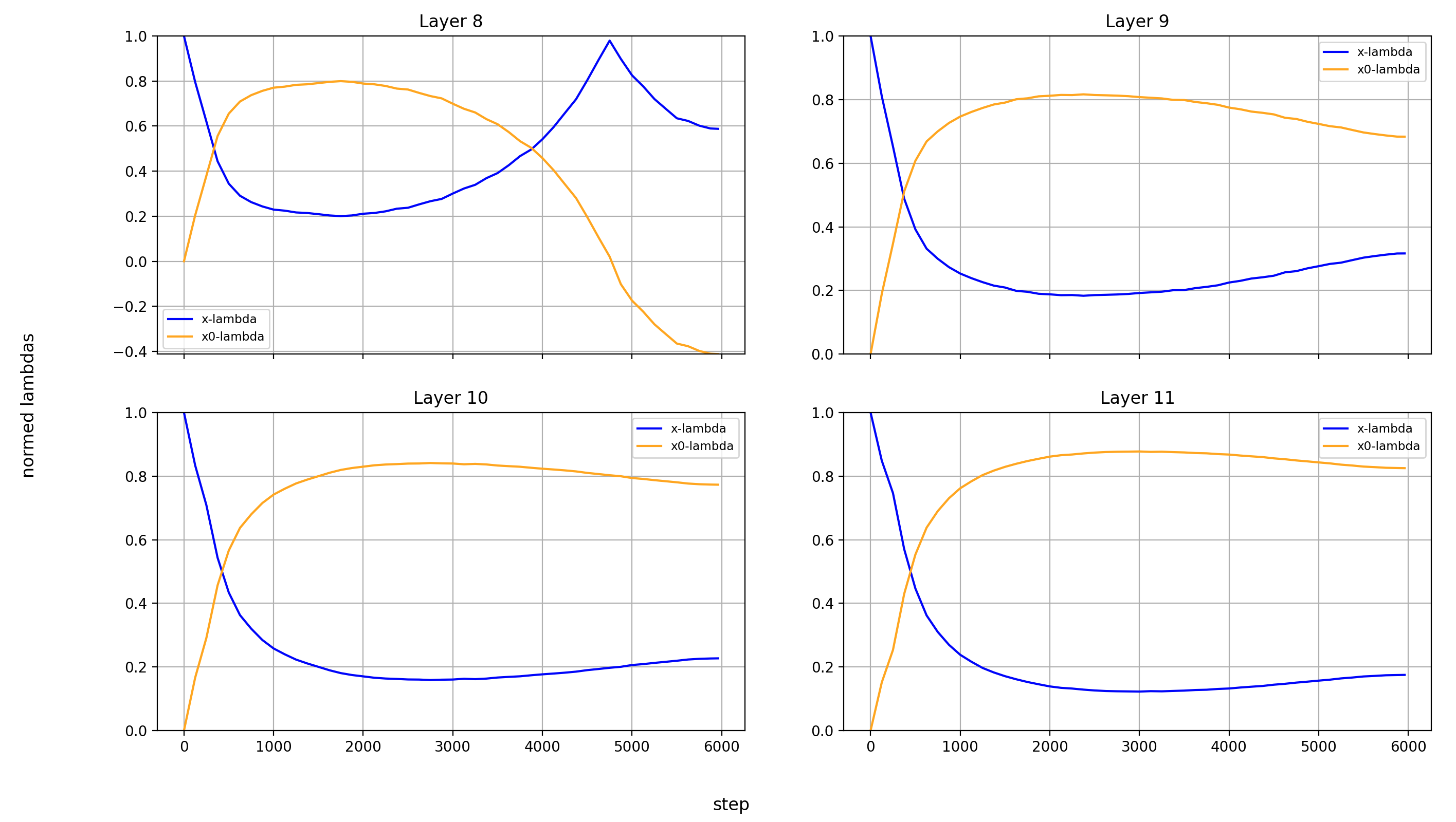
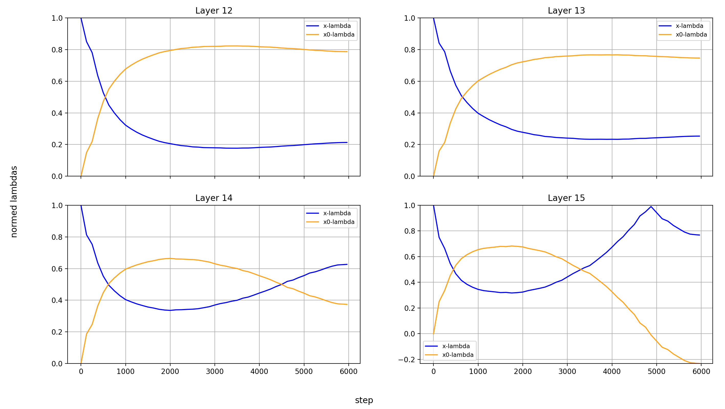
What immediately jumps out to me is that in layers 8, 14, and 15, x0_lambda first grows relative to x_lambda, before dropping off a cliff and crossing over into negative territory. That means that for a short while, it’s at 0, and x0 has no impact on these three layers.
It’s also curious to me that the crossover into negative values happens so late in training. That means that it happens when the model is already used to a positive x0_lambda in these layers. Inverting the sign of the x0 summand changes the embedding math, and that points to something else changing at the same time.
This change doesn’t cause any loss spikes though, the validation loss is smooth as ever:

What’s also interesting is that layer 14 is the only layer in which x0_lambda remains positive at the end of training, while still being lower than x_lambda.
Another phenomenon is that the impact of x0 rises over most of training, and then falls again at the end, in every single layer but the first (where it doesn’t matter). This tends to happen earlier than the crossover of x0_lambda into negative values in layers 8 and 15.
I wonder how these dynamics are connected to the learning rate schedule and the sequence length schedule (modded-nanogpt uses a block mask that increases in size over the course of training). So here is a plot of the learning rate and sequence length, relative to their absolute values (so normalized to between 0 and 1):

The learning rate is constant for the first ~2000 steps, then falls linearly to 0. The sequence length rises to half its maximum in the first ~2000 steps, then remains constant for ~2000 steps, before rising again in the last ~2000 steps.
And that is indeed very informative!
- The impact of x0 stops rising relative to x right around the time when the learning rate begins decaying, and the sequence length becomes constant
- In layer 14, x becomes more important than x0 right after the sequence length begins increasing again
- The
x0_lambdacrossover happens shortly after that, which makes it look like it is also connected to the sequence length schedule
The last two points make a lot of sense to me: the solution to an increasing sequence length is to move away more strongly from x0, which provides a bias toward the immediate neighborhood of each token. That can then be adjusted later on as the weights are updated, but it’s a really logical step at least for a while.
I don’t know how meaningful these are, and how consistent they happen over different training runs, but the close relationship between hyperparameters and x0-lambdas make me think that there are real phenomena here.
Here are some more observations:
One interesting phenomenon is that the early layers tend to have higher absolute x0_lambda values than the later ones, which means two things:
- The early layers make really small adjustments to the input embeddings
- x0 is carried to the later layers with more weight through the U-Net connections
Taking the U-Net connections into account, these very high absolute values means thats the effective model depth is shortened again, and middle layers add their algorithmic complexity in more subtle ways.
But it might also be connected with the value embeddings, which are applied to the first and last three layers. High x- and x0-magnitudes in the first three layers suppress the relative impact of the value embeddings, while low magnitudes in the last layers will keep them high. But let’s re-visit this later.
Layers 8 and 15 are the layers with the lowest x_lambda and x0_lambda. I’m not sure what that means, just wanted to point it out.
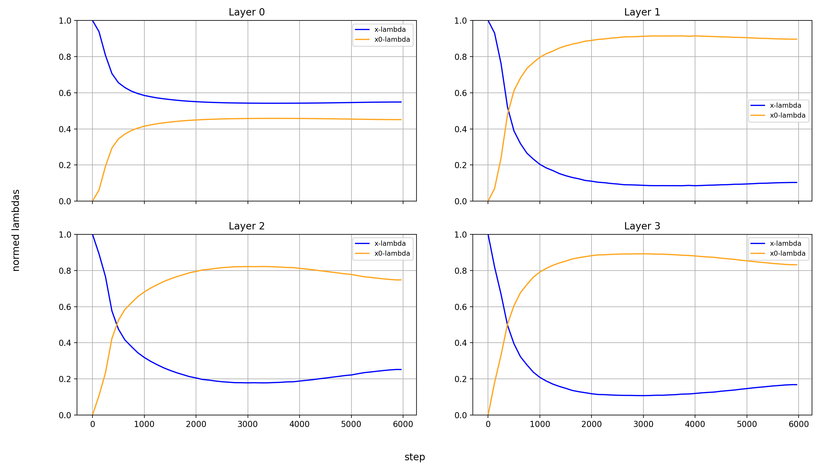
For the sake of completeness, here are also the normalized values:
Value-Embeddings Lambdas
The value embeddings are embedding layers beside the one that forms x0. Their embeddings are added to the Values in the causal self-attention block right before flexattention is applied: v = v_lambda * v + ve_lambda * ve.view_as(v) (where ve are the layer’s value embeddings)
However, that is only the case in the first and last three layers. In between, only v_lambda is used to scale the Values, while ve_lambda remains unchanged over training. And at layer 7, there is no attention, so there are no such lambdas.
To add more complexity, the value embeddings of the first and last three layers are shared; so layers 0 and 13, layers 1 and 14, and layers 2 and 15 share the same value embeddings. This saves parameters and ensures that there is a short gradient path from the loss to the value embeddings. While additional gradient comes from the first three layers which are the farthest away from the input, there is always gradient from the three layers nearest to the loss, too.
I admit that I only have some very weak intuitions for why value embeddings help. I’ve long held that token embeddings are a way to hold training-set wide statistics about the byte-sequence represented by the token, so I’m guessing that they add a way for the model to store more static per-token statistics which are helpful. Another viewpoint on this is that at least the value embeddings at the last three layers effectively reduce the model depth again. The most basic idea is that embeddings in general are a very cheap way to add parameters to an LLM (because they don’t require a matrix multiplication, just a lookup). And finally, as discussed above, the value embeddings act as a learned, data-dependent bias term. However, that’s 100% speculation and you shouldn’t take it too seriously.
More importantly, I will again plot the final values of these lambdas over the layers. And this time both the absolute and the relative values are of interest. The absolute values are specifically interesting for the layers in which there are no value-embeddings but v_lambda is still used to scale the values. The normed values are particularly interesting (at least in my eyes) for the layers where values embeddings are applied, because I’m interested in their weight relative to the values.
So here is the plot with the absolute values:

Some observations about the layers without value embeddings (layers 3-12):
- The model really likes to scale the attention-values by around 6-7 via
v_lambda - There seems to be a trend to do this more strongly in the later layers, but it’s weak and I don’t know if it’s meaningful
- At these layers,
ve_lambdaof course stays unchanged throughout training, because it’s never used
Some observations about the layer with value embeddings (layers 0-2 and 13-15):
v_lambdais significantly larger than at initialization for all layers, though not as much as without value embeddingsve_lambdastays very low, except in the last layer- The ratio of
v_lambdatove_lambdais much higher in the first than the last layers; the value embeddings seem to have little impact on the first few layers (at least numerically, they could still stabilize training, or add just enough to make a difference, or whatever, but this is only supported by the high magnitudes of x0 from the x0-lambdas).
To make more sense of that last point especially, let’s look at the normalized lambdas:

Three clear groups emerge:
- Layers 0-2, which are affected very weakly by the value embeddings (by only around 10%)
- Layers 13 and 14, which are affected fairly strongly by the value embeddings (by around 25%)
- Layer 15, which uses its value embeddings almost as strongly as its input from the residual stream (with around 45% intensity)
Let’s look at the lambdas over the course of training again.
First the normalized values:


In the layers without value embeddings, the magnitude of the attention-values rises very quickly and never reverses course.
But in the layer with value embeddings, only layers 0 and 1 behave like that. For layers 2 and 13-15, the value embeddings first gain in relative importance before losing it again. The later the layer, the later this reversal happens.
And here are the un-normed values:


In all layers, the v_lambdas rise over most of training, before slightly falling toward the end.
Summary
I’ve ran the modded-nanogpt medium track training once (so don’t overindex on this) and plotted all the scalar values that are being trained. Hope you enjoyed.
Citation
@misc{snimu2025lambdas,
    title={modded-nanogpt: Analyzing value-embedding-, UNet-, and x0-lambdas},
    author={Sebastian Nicolas Müller},
    year={2025},
    month={08},
    url={https://snimu.github.io/2025/08/11/modded-nanogpt-lambdas.html}
}